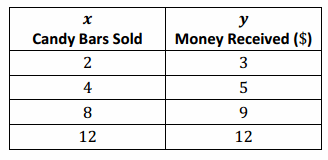
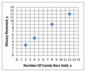
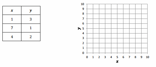
Isaiah sold candy bars to help raise money for his scouting troop. The table shows the amount of candy he sold compared to the money he received Is the amount of candy bars sold proportional to the money Isaiah received? How do you know? ___________________________________________________________________ Answer: The two quantities are not proportional to each other because a constant describing the proportion does not exist.
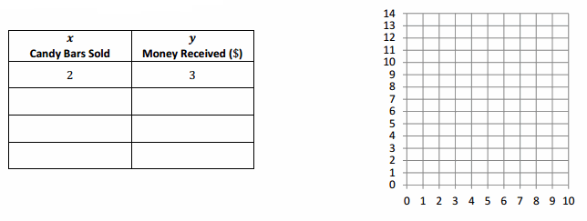
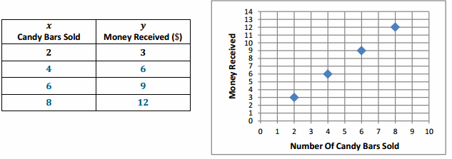
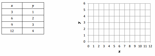
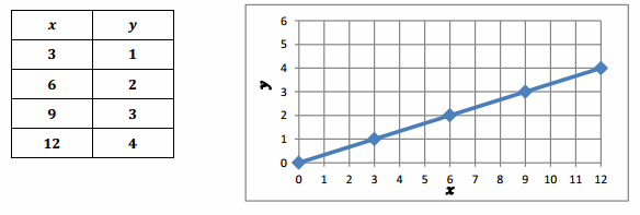
From a Table to a Graph Using the ratio provided, create a table that shows that money received is proportional to the number of candy bars sold. Plot the points in your table on the grid. Answer:
Eureka Math Grade 7 Module 1 Lesson 5 Problem Set Answer Key
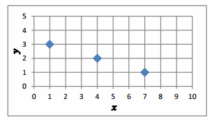
Example 1. Graph the points from the Opening Exercise. Answer:
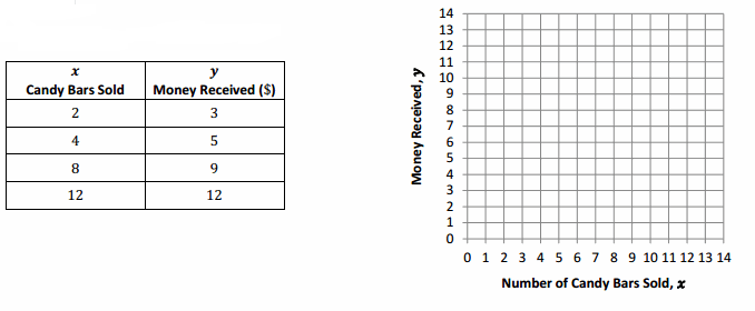
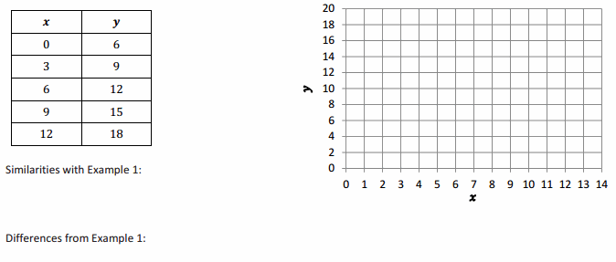
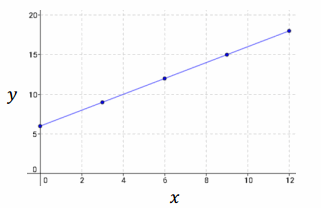
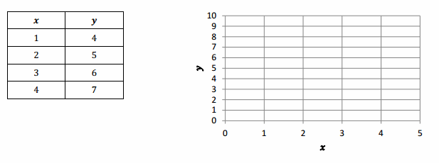
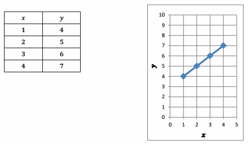
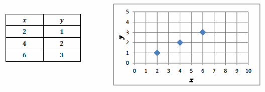
Example 2. Graph the points provided in the table below, and describe the similarities and differences when comparing your graph to the graph in Example 1. Answer:
Similarities with Example 1: Answer: The points of both graphs fall in a line.
Differences from Example 1: Answer: The points of the graph in Example 1 appear on a line that passes through the origin. The points of the graph in Example 3 appear on a line that does not pass through the origin.
Eureka Math Grade 7 Module 1 Lesson 5 Problem Set Answer Key
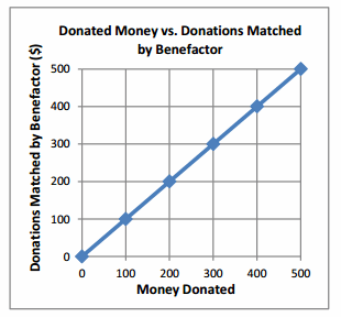
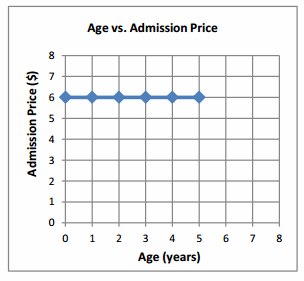
Question 1. Determine whether or not the following graphs represent two quantities that are proportional to each other. Explain your reasoning. a. Answer: This graph represents two quantities that are proportional to each other because the points appear on a line, and the line that passes through the points would also pass through the origin.
b. Answer: Even though the points appear on a line, the line does not go through the origin. Therefore, this graph does not represent a proportional relationship.
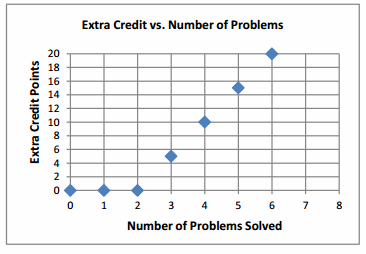
c. Answer: Even though it goes through the origin, this graph does not show a proportional relationship because the points do not appear on one line.
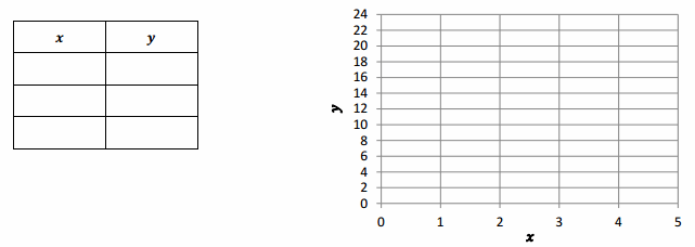
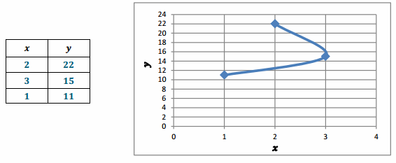
Question 2. Create a table and a graph for the ratios 2:22, 3 to 15, and 1:11. Does the graph show that the two quantities are proportional to each other? Explain why or why not. Answer: This graph does not because the points do not appear on a line that goes through the origin.
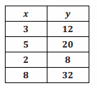
Question 3. Graph the following tables, and identify if the two quantities are proportional to each other on the graph. Explain why or why not. a. Answer: Yes, because the graph of the relationship is a straight line that passes through the origin.
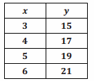
b. Answer: No, because the graph does not pass through the origin.
Question 1. The following table gives the number of people picking strawberries in a field and the corresponding number of hours that those people worked picking strawberries. Graph the ordered pairs from the table. Does the graph represent two quantities that are proportional to each other? Explain why or why not. Answer: Although the points fall on a line, the line does not pass through the origin, so the graph does not represent two quantities that are proportional to each other.
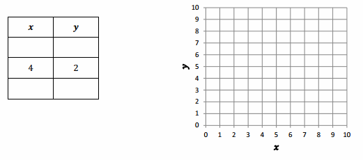
Question 2. Use the given values to complete the table. Create quantities proportional to each other and graph them. Answer:
Question 3. a. What are the differences between the graphs in Problems 1 and 2? Answer: The graph in Problem 1 forms a line that slopes downward, while the graph in Problem 2 slopes upward.
b. What are the similarities in the graphs in Problems 1 and 2? Answer: Both graphs form lines, and both graphs include the point (4,2).
c. What makes one graph represent quantities that are proportional to each other and one graph not represent quantities that are proportional to each other in Problems 1 and 2? Answer: Although both graphs form lines, the graph that represents quantities that are proportional to each other needs to pass through the origin.
Engage NY Eureka Math 7th Grade Module 1 Lesson 4 Answer Key
Eureka Math Grade 7 Module 1 Lesson 4 Example Answer Key
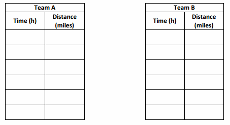
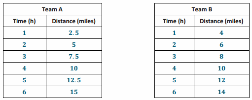
Which Team Will Win the Race? You have decided to walk in a long-distance race. There are two teams that you can join. Team A walks at a constant rate of 2.5 miles per hour. Team B walks 4 miles the first hour and then 2 miles per hour after that. Task: Create a table for each team showing the distances that would be walked for times of 1, 2, 3, 4, 5, and 6 hours. Using your tables, answer the questions that follow. Answer:
a. For which team is distance proportional to time? Explain your reasoning. Answer: Distance is proportional to time for Team A since all the ratios comparing distance to time are equivalent. The value of each ratio is 2.5. Every measure of time can be multiplied by 2.5 to give the corresponding measures of distance.
b. Explain how you know the distance for the other team is not proportional to time. Answer: For Team B, the ratios are not equivalent. The values of the ratios are 4, 3, \(\frac{8}{3}\), \(\frac{5}{2}\), \(\frac{12}{5}\), and \(\frac{7}{3}\). Therefore, every measure of time cannot be multiplied by a constant to give each corresponding measure of distance.
c. At what distance in the race would it be better to be on Team B than Team A? Explain. Answer: If the race were fewer than 10 miles, Team B is faster because more distance would be covered in less time.
d. If the members on each team walked for 10 hours, how far would each member walk on each team? Answer: Team A = 25 miles Team B = 22 miles
e. Will there always be a winning team, no matter what the length of the course? Why or why not? Answer: No, there would be a tie (both teams win) if the race were 10 miles long. It would take each team 4 hours to complete a 10-mile race.
f. If the race were 12 miles long, which team should you choose to be on if you wish to win? Why would you choose this team? Answer: I should choose Team A because they would finish in 4.8 hours compared to Team B finishing in 5 hours.
g. How much sooner would you finish on that team compared to the other team? Answer: \(\frac{2}{10}\) of an hour or \(\frac{2}{10}\)(60) = 12 minutes
Bella types at a constant rate of 42 words per minute. Is the number of words she can type proportional to the number of minutes she types? Create a table to determine the relationship. Answer: This relationship is proportional because I can multiply the number of minutes by the constant to get the corresponding number of words. The value of the ratio is 42. The constant is also 42.
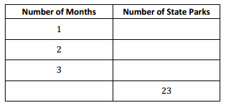
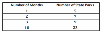
Question 2. Mark recently moved to a new state. During the first month, he visited five state parks. Each month after, he visited two more. Complete the table below, and use the results to determine if the number of parks visited is proportional to the number of months Answer: This relationship is not proportional. There is no constant value that can be multiplied by the number of months to get the corresponding number of parks visited.
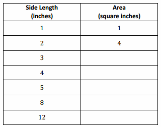
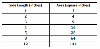
Question 3. The table below shows the relationship between the side length of a square and the area. Complete the table. Then, determine if the length of the sides is proportional to the area. Answer: This relationship is not proportional. There is no constant value that can be multiplied by the side length to get the corresponding area.
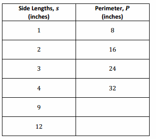
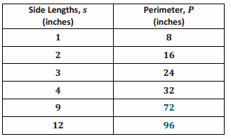
The table below shows the relationship between the side lengths of a regular octagon and its perimeter. Complete the table. If Gabby wants to make a regular octagon with a side length of 20 inches using wire, how much wire does she need? Justify your reasoning with an explanation of whether perimeter is proportional to the side length. Answer: 20(8)=160 Gabby would need 160 inches of wire to make a regular octagon with a side length of 20 inches. This table shows that the perimeter is proportional to the side length because the constant is 8, and when all side lengths are multiplied by the constant, the corresponding perimeter is obtained. Since the perimeter is found by adding all 8 side lengths together (or multiplying the length of 1 side by 8), the two numbers must always be proportional.
Eureka Math Grade 7 Module 1 Lesson 4 Problem Set Answer Key
Question 1. Joseph earns $15 for every lawn he mows. Is the amount of money he earns proportional to the number of lawns he mows? Make a table to help you identify the type of relationship. Answer: The table shows that the earnings are proportional to the number of lawns mowed. The value of each ratio is 15. The constant is 15.
Question 2. At the end of the summer, Caitlin had saved $120 from her summer job. This was her initial deposit into a new savings account at the bank. As the school year starts, Caitlin is going to deposit another $5 each week from her allowance. Is her account balance proportional to the number of weeks of deposits? Use the table below. Explain your reasoning. Answer: Caitlin’s account balance is not proportional to the number of weeks because there is no constant such that any time in weeks can be multiplied to get the corresponding balance. In addition, the ratio of the balance to the time in weeks is different for each column in the table. 120:0 is not the same as 125:1.
Question 3. Lucas and Brianna read three books each last month. The table shows the number of pages in each book and the length of time it took to read the entire book.
a. Which of the tables, if any, represent a proportional relationship? Answer: The table shows Lucas’s number of pages read to be proportional to the time because when the constant of 26 is multiplied by each measure of time, it gives the corresponding values for the number of pages read.
b. Both Lucas and Brianna had specific reading goals they needed to accomplish. What different strategies did each person employ in reaching those goals? Answer: Lucas read at a constant rate throughout the summer, 26 pages per hour, whereas Brianna’s reading rate was not the same throughout the summer.
Engage NY Eureka Math 7th Grade Module 1 Lesson 3 Answer Key
Eureka Math Grade 7 Module 1 Lesson 3 Example Answer Key
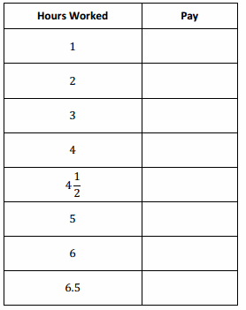
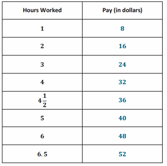
Example You have been hired by your neighbors to babysit their children on Friday night. You are paid $8 per hour. Complete the table relating your pay to the number of hours you worked. Answer: Based on the table above, is the pay proportional to the hours worked? How do you know? Answer: Yes, the pay is proportional to the hours worked because every ratio of the amount of pay to the number of hours worked is the same. The ratio is 8:1, and every measure of hours worked multiplied by 8 will result in the corresponding measure of pay.
For Exercises 1–3, determine if y is proportional to x. Justify your answer.
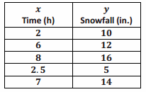
Question 1. The table below represents the relationship of the amount of snowfall (in inches) in 5 counties to the amount of time (in hours) of a recent winter storm. Answer: y (snowfall) is not proportional to x (time) because all of the values of the ratios comparing snowfall to time are not equivalent. All of the values of the ratios must be the same for the relationships to be proportional. There is NOT one number such that each measure of x (time) multiplied by the number gives the corresponding measure of y (snowfall).
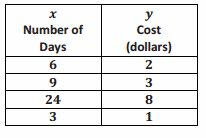
Question 2. The table below shows the relationship between the cost of renting a movie (in dollars) to the number of days the movie is rented. Answer: y (cost) is proportional to x (number of days) because all of the values of the ratios comparing cost to days are equivalent. All of the values of the ratios are equal to \(\frac{1}{3}\). Therefore, every measure of x (days) can be multiplied by the number \(\frac{1}{3}\) to get each corresponding measure of y (cost).
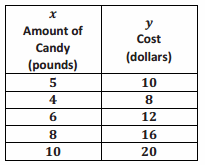
Question 3. The table below shows the relationship between the amount of candy bought (in pounds) and the total cost of the candy (in dollars). Answer: y(cost) is proportional to ????(amount of candy) because all of the values of the ratios comparing cost to pounds are equivalent. All of the values of the ratios are equal to ???? Therefore, every measure of x (amount of candy) can be multiplied by the number 2 to get each corresponding measure of y (cost).
Possible questions asked by the teacher or students:
→When looking at ratios that describe two quantities that are proportional in the same order, do the ratios always have to be equivalent?
→ Yes, all the ratios are equivalent, and a constant exists that can be multiplied by the measure of the first quantity to get the measure of the second quantity for every ratio pair.
→ For each example, if the quantities in the table were graphed, would the point (0,0) be on that graph? Describe what the point (0,0) would represent in each table.
→ Exercise 1: 0 inches of snowfall in 0 hours
→ Exercise 2: Renting a movie for 0 days costs $0
→ Exercise 3: 0 pounds of candy costs $0
→ Do the x- and y-values need to go up at a constant rate? In other words, when the x- and y-values both go up at a constant rate, does this always indicate that the relationship is proportional?
→ Yes, the relationship is proportional if a constant exists such that each measure of the x when multiplied by the constant gives the corresponding y-value.
Question 4. Randy is driving from New Jersey to Florida. Every time Randy stops for gas, he records the distance he traveled in miles and the total number of gallons he used. Assume that the number of miles driven is proportional to the number of gallons consumed in order to complete the table. Answer: Since the quantities are proportional, then every ratio comparing miles driven to gallons consumed must be equal. Using the given values for each quantity, the value of the ratio is \(\frac{54}{2}\) = 27 \(\frac{216}{8}\)=27
If the number of gallons consumed is given and the number of miles driven is the unknown, then multiply the number of gallons consumed by 27 to determine the number of miles driven. 4(27)=108 10(27)=270 12(27)=324
If the number of miles driven is given and the number of gallons consumed is the unknown, then divide the number of miles driven by 27 to determine the number of gallons consumed. \(\frac{189}{27}\) = 7
→ Why is it important for you to know that the number of miles are proportional to the number of gallons used?
→Without knowing this proportional relationship exists, just knowing how many gallons you consumed will not allow you to determine how many miles you traveled. You would not know if the same relationship exists for each pair of numbers.
→Describe the approach you used to complete the table.
→ Since the number of miles driven is proportional to the number of gallons consumed, a constant exists such that every measure of gallons used can be multiplied by the constant to give the corresponding amount of miles driven. Once this constant is found to be 27, it can be used to fill in the missing parts by multiplying each number of gallons by 27.
→ What is the value of the constant? Explain how the constant was determined.
→ The value of the constant is 27. This was determined by dividing the given number of miles driven by the given number of gallons consumed.
→ Explain how to use multiplication and division to complete the table.
→ If the number of gallons consumed was given, then that number is to be multiplied by the constant of 27 to determine the amount of the miles driven. If the number of miles driven were given, then that number needs to be divided by the constant of 27 to determine the number of gallons consumed.
The table below shows the price, in dollars, for the number of roses indicated.
Question 1. Is the price proportional to the number of roses? How do you know? Answer: The quantities are proportional to one another because there is a constant of 3 such that when the number of roses is multiplied by the constant, the result is the corresponding price.
Question 2. Find the cost of purchasing 30 roses. Answer: If there are 30 roses, then the cost would be 30×3=$90.
Eureka Math Grade 7 Module 1 Lesson 3 Problem Set Answer Key
In each table, determine if y is proportional to x. Explain why or why not.
Question 1. Yes, y is proportional to x because the values of all ratios of \(\frac{y}{x}\) are equivalent to 4. Each measure of x multiplied by this constant of 4 gives the corresponding measure in y.
Question 2. Answer: No, y is not proportional to x because the values of all the ratios of \(\frac{y}{x}\) are not equivalent. There is not a constant where every measure of x multiplied by the constant gives the corresponding measure in y. The values of the ratios are 5, 4.25, 3.8, and 3.5.
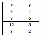
Question 3. Answer: Yes, y is proportional to x because a constant value of \(\frac{2}{3}\) exists where each measure of x multiplied by this constant gives the corresponding measure in y.
Question 4. Kayla made observations about the selling price of a new brand of coffee that sold in three different-sized bags. She recorded those observations in the following table:
Ounces of Coffee
Price in Dollars
a. Is the price proportional to the amount of coffee? Why or why not? Answer: Yes, the price is proportional to the amount of coffee because a constant value of 0.35 exists where each measure of x multiplied by this constant gives the corresponding measure in y.
b. Use the relationship to predict the cost of a 20 oz. bag of coffee. Answer: 20 ounces will cost $7.
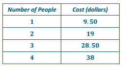
Question 5. you and your friends go to the movies. The cost of admission is $9.50 per person. Create a table showing the relationship between the number of people going to the movies and the total cost of admission. Explain why the cost of admission is proportional to the amount of people. Answer: The cost is proportional to the number of people because a constant value of 9.50 exists where each measure of the number of people multiplied by this constant gives the corresponding measure in y.
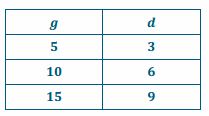
Question 6. For every 5 pages Gil can read, his daughter can read 3 pages. Let g represent the number of pages Gil reads, and let d represent the number of pages his daughter reads. Create a table showing the relationship between the number of pages Gil reads and the number of pages his daughter reads. Is the number of pages Gil’s daughter reads proportional to the number of pages he reads? Explain why or why not. Answer: Yes, the number of pages Gil’s daughter reads is proportional to the number of pages Gil reads because all the values of the ratios are equivalent to 0.6. When I divide the number of pages Gil’s daughter reads by the number of pages Gil reads, I always get the same quotient. Therefore, every measure of the number of pages Gil reads multiplied by the constant 0.6 gives the corresponding values of the number of pages Gil’s daughter’s reads.
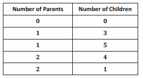
Question 7. The table shows the relationship between the number of parents in a household and the number of children in the same household. Is the number of children proportional to the number of parents in the household? Explain why or why not. Answer: No, there is not a proportional relationship because there is no constant such that every measure of the number of parents multiplied by the constant would result in the corresponding values of the number of children. When I divide the number of children by the corresponding number of parents, I do not get the same quotient every time. Therefore, the values of the ratios of children to parents are not equivalent. They are 3, 5, 2, and 0.5.
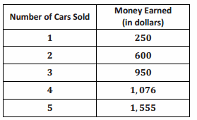
Question 8. The table below shows the relationship between the number of cars sold and the amount of money earned by the car salesperson. Is the amount of money earned, in dollars, proportional to the number of cars sold? Explain why or why not. Answer: No, there is no constant such that every measure of the number of cars sold multiplied by the constant would result in the corresponding values of the earnings because the ratios of money earned to number of cars sold are not equivalent; the values of the ratios are 250, 300, 316\(\frac{2}{3}\), 269, and 311.
Question 9. Make your own example of a relationship between two quantities that is NOT proportional. Describe the situation, and create a table to model it. Explain why one quantity is not proportional to the other Answer: Answers will vary but should include pairs of numbers that do not always have the same value \(\frac{B}{A}\).
Engage NY Eureka Math 7th Grade Module 1 Lesson 2 Answer Key
Eureka Math Grade 7 Module 1 Lesson 2 Example Answer Key
Example 1. Pay by the Ounce Frozen Yogurt The purpose of this example is for students to understand when measures of one quantity are proportional to measures of another quantity. Answer: A new self-serve frozen yogurt store opened this summer that sells its yogurt at a price based upon the total weight of the yogurt and its toppings in a dish. Each member of Isabelle’s family weighed his dish, and this is what they found. Determine if the cost is proportional to the weight.
Weight (ounces)
Cost ($)
The cost _____________________________________ the weight.
Discuss the following questions:
→ Does everyone pay the same cost per ounce? How do you know?
→ Yes, it costs $0.40 per ounce. If we divide each cost value by its corresponding weight, it will give the same unit price (or unit rate) of 0.40. Since we want to compare cost per ounce, we can use the unit (cost per ounce) to determine that we want to divide each cost value by each corresponding weight value.
→ Isabelle’s brother takes an extra-long time to create his dish. When he puts it on the scale, it weighs 15 ounces. If everyone pays the same rate in this store, how much will his dish cost? How did you calculate this cost?
→ $6. I determined the cost by multiplying 0.40 by 15 ounces.
→ Since this is true, we say “the cost is proportional to the weight.” Complete the statement in your materials.
→What happens if you don’t serve yourself any yogurt or toppings? How much do you pay?
→ $0.
→ Does the relationship above still hold true? In other words, if you buy 0 ounces of yogurt, then multiply by the cost per ounce, do you get 0?
→ Even for 0, you can still multiply by this constant value to get the cost (not that you would do this, but we can examine this situation for the sake of developing a rule that is always true).
→ Always multiply the number of ounces, x, by the constant that represents cost per ounce to get the total cost, y. Pause with students to note that any variables could be chosen but that for the sake of this discussion, they are x and y.
The teacher should label the table with the indicated variables and guide students to do the same.
→ For any measure x, how do we find y?
→ Multiply it by 0.40 (unit price).
→ Indicate this on the given chart, as done below. Be sure students do the same.
→ So, y = 0.40x.
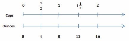
Example 2. A Cooking Cheat Sheet In the back of a recipe book, a diagram provides easy conversions to use while cooking.
The ounces _____________________________________the cups. Answer:
What does the diagram tell us?
The number of ounces in a given number of cups. More specifically, each pair of numbers indicates the correct matching of ounces to cups.
Is the number of ounces proportional to the number of cups? How do you know?
Yes, you can multiply each number of cups by 8 to get the number of ounces.
Have students complete the statement on their materials, ounces is proportional to cups, and note how they can tell. It is important to acknowledge that they could also divide by 8 if they know the number of ounces and are trying to find the number of cups. This discussion should lead to the importance of defining the quantities clearly.
How many ounces are there in 4 cups? 5 cups? 8 cups? How do you know?
32, 40, 64; each time, the number of cups is multiplied by 8 to get the number of ounces.
For the sake of this discussion (and to provide continuity between examples), let’s represent the cups with x, and the ounces with y.
The teacher should label the diagram with the indicated variables and guide students to do the same.
For any number of cups x, how do we find the number of ounces, y?
Multiply x by 8.
So, y=8x.
If we want to verify that our equation is y=8x, which x and y values can we use to see if it is true? How do you know?
We can choose any pair of given (x,y) values since the equation should model the relationship for every pair of values.
It is a good idea to check more than one pair. Guide students to substitute the pairs of values into the equation to prove that for each one, the equation is true.
Example 3: Summer Job Alex spent the summer helping out at his family’s business. He was hoping to earn enough money to buy a new $220 gaming system by the end of the summer. Halfway through the summer, after working for 4 weeks, he had earned $112. Alex wonders, “If I continue to work and earn money at this rate, will I have enough money to buy the gaming system by the end of the summer?” To determine if he will earn enough money, he decided to make a table. He entered his total money earned at the end of Week 1 and his total money earned at the end of Week 4.
a. Work with a partner to answer Alex’s question. Answer: Yes, Alex will have earned enough money to buy the $220 gaming system by the end of the summer because he will have earned 8∙28, or 224 dollars, for the 8 weeks he worked. A sample table is shown below.
Allow for students to share responses with the class for part (b), and then record in their student pages.
b. Are Alex’s total earnings proportional to the number of weeks he worked? How do you know? Answer: Alex’s total earnings are proportional to the number of weeks he worked. There exists a constant value, 28, which can be multiplied by the number of weeks to determine the corresponding earnings for that week. The table shows an example of a proportional relationship.
Exercise 1. Have students complete the following example independently, and then discuss responses as a class.
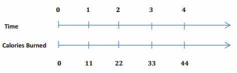
During Jose’s physical education class today, students visited activity stations. Next to each station was a chart depicting how many calories (on average) would be burned by completing the activity. Calories Burned While Jumping Rope
a. Is the number of calories burned proportional to time? How do you know? Answer: Yes, the time is always multiplied by the same number, 11, to find the calories burned.
b. If Jose jumped rope for 6.5 minutes, how many calories would he expect to burn? Answer: Jose would expect to burn 71.5 calories since 6.5 times 11 is 71.5.
Ms. Albero decided to make juice to serve along with the pizza at the Student Government party. The directions said to mix 2 scoops of powdered drink mix with a half gallon of water to make each pitcher of juice. One of Ms. Albero’s students said she will mix 8 scoops with 2 gallons of water to make 4 pitchers. How can you use the concept of proportional relationships to decide whether the student is correct? Answer: As long as the amount of water is proportional to the number of scoops of drink mix, then the second quantity, amount of water, can be determined by multiplying the first quantity by the same constant. In this case, if the amount of powdered drink mix is represented by x, and the gallons of water are represented by y, then y = \(\frac{1}{4}\) x. To determine any of the measures of water, you will multiply the number of scoops by \(\frac{1}{4}\).
Eureka Math Grade 7 Module 1 Lesson 2 Problem Set Answer Key
Question 1. A cran-apple juice blend is mixed in a ratio of cranberry to apple of 3 to 5. a. Complete the table to show different amounts that are proportional. Answer:
b. Why are these quantities proportional? Answer: The amount of apple is proportional to the amount of cranberry since there exists a constant number, \(\frac{5}{3}\), that when multiplied by any of the given measures for the amount of cranberry always produces the corresponding amount of apple. If the amount of cranberry is represented by x, and the amount of apple is represented by y, then each pair of quantities satisfies the equation y = \(\frac{5}{3}\)x. A similar true relationship could be derived by comparing the amount of cranberry to the amount of apple. In the case where x is the amount of apple and y is the amount of cranberry, the equation would be y = \(\frac{3}{5}\)x.
Question 3 John is filling a bathtub that is 18 inches deep. He notices that it takes two minutes to fill the tub with three inches of water. He estimates it will take 10 more minutes for the water to reach the top of the tub if it continues at the same rate. Is he correct? Explain.
Time (minutes)
Bathtub Water Height (inches)
Answer: Yes. In 10 more minutes, the tub will reach 18 inches. At that time, the ratio of time to height may be expressed as 12 to 18, which is equivalent to 2 to 3. The height of the water in the bathtub increases 1\(\frac{1}{2}\) inches every minute.
Engage NY Eureka Math 7th Grade Module 1 Lesson 1 Answer Key
Eureka Math Grade 7 Module 1 Example Answer Key
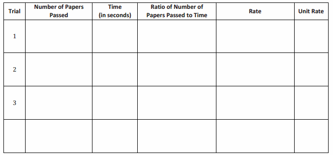
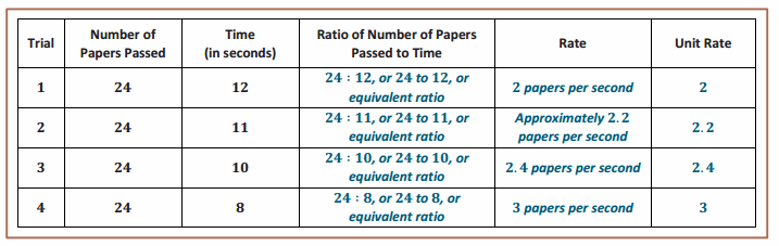
Example 1. How Fast Is Our Class? Record the results from the paper-passing exercise in the table below.
Key Terms from Grade 6 Ratios and Unit Rates
A ratio is an ordered pair of numbers which are not both zero. A ratio is denoted A : B to indicate the order of the numbers: the number is first, and the number is second.
Two ratios A : B and C : D are equivalent ratios if there is a nonzero number c such that C = cA and D = cB. For example, two ratios are equivalent if they both have values that are equal.
A ratio relationship between two types of quantities, such as 5 miles per 2 hours, can be described as a rate (i.e., the quantity 2.5 miles/hour).
The numerical part of the rate is called the unit rate and is simply the value of the ratio, in this case 2.5. This means that in 1 hour the car travels 2.5 miles. The unit for the rate is miles/hour, read miles per hour.
Answer: To start this first class of the school year, conduct an exercise in how to pass out papers. The purpose of the task is not only to establish a routine at the start of the school year but also to provide a context to discuss ratio and rate.
Determine how papers will be passed out in class depending upon seating arrangement. For this task, it is best to divide the original stack so that one student (in each row or group) has a portion of the original stack. Based upon this determination, explain the system to students. A brief demonstration may help to provide a visual.
For example: If the room is arranged in rows, pass across the rows. Have students start on command and perhaps require that only the current paper-passing student may be out of his or her seat. If the room is arranged in groups or at tables, have the students pass papers to their left, on command, until everyone has a paper. Note: This procedure is highly customizable for use in any classroom structure.
Begin the task by handing a stack of papers to a starting person. Secretly start a stopwatch as the start command is given. Once every student has a paper, report the paper-passing time out loud. For example, “It took 12 seconds. Not bad, but let’s see if we can get these papers passed out in 11 seconds next time.”
Tell students to begin returning papers back in to the original stack, and then report the time upon completion.
Excellent job. Now, pass them back out in 10 seconds. Excellent. Now, pass them back in 8 seconds. Pose the following questions to the students as a whole group, one question at a time.
How will we measure our rate of passing out papers?
Using a stopwatch or similar tool to measure the number of seconds taken to pass out papers.
What quantities will we use to describe our rate?
The number of papers passed out and the time that it took to pass them out.
Complete the second and third columns (number of papers and time) on the table as a class.
Describe the quantities you want to measure by talking about what units we use to measure each quantity.
One quantity measures the number of papers, and the other measures the number of seconds.
Review the Key Terms box defining ratio, rate, and unit rate in the student materials. Focus on reviewing the concept of ratio first, perhaps using a few quick examples.
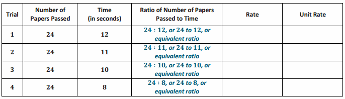
Guide students to complete the ratio column in the table as shown below. Record the results from the paper-passing exercise in the table below.
When we started passing papers, the ratio of the number of papers to the number of seconds was 24 to 12, and by the end of the activity, the ratio of the number of papers to the number of seconds was 24 to 8. Are these two ratios equivalent? Explain why or why not.
Guide students in a discussion about the fact that the number of papers was constant, and the time decreased with each successive trial. See if students can relate this to rate and ultimately determine which rate is greatest.
The ratios are not equivalent since we passed the same number of papers in a shorter time. We passed 2 papers per second at the beginning and 3 papers per second by the end. Equivalent ratios must have the same value.
The following questioning is meant to guide students into the realization that unit rate helps us to make comparisons between a variety of ratios and compare different data points.
In another class period, students were able to pass 28 papers in 15 seconds, and then 28 papers in 12 seconds. A third class period passed 18 papers in 10 seconds. How do these compare to our class?
Use sample data here, or use real data collected from other classes prepared in advance.
We could find how many papers were passed per second to make these comparisons. Answers on how they compare would vary depending on class results in the table.
Review the meaning of rate and unit rate in the Key Terms box, and complete the last two columns of the table, modeling how to find both rate and unit rate. The associated unit rate is the numerical value \(\frac{A}{B}\) when there are A units of one quantity for every B units of another quantity.
Example 2: Our Class by Gender
Number of Boys
Number of Girls
Ratio of Boys to Girls
Class 1
Class 2
Whole 7th Grade
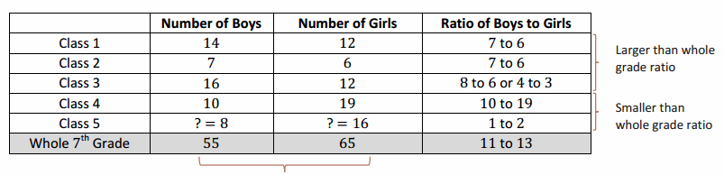
Create a pair of equivalent ratios by making a comparison of quantities discussed in this Example. Answer: Let’s make a comparison of two quantities that are measured in the same units by comparing the ratio of the number of boys to the number of girls in this class to the ratio for different classes (and the whole grade). Sample discussion:
In this class, we have 14 boys and 12 girls. In another class, there are 7 boys and 6 girls. Note: Any class may be used for comparison; the ratios do not need to be equivalent.
Guide students to complete the table accordingly, pausing to pose the questions below.
Number of Boys
Number of Girls
Ratio of Boys to Girls
Class 1
14
12
7 to 6
Class 2
7
6
7 to 6
Whole 7th Grade
Answers vary
Answers vary
create a pair of equivalent ratios by making a comparison of quantities discussed in this example.
Are the ratios of boys to girls in the two classes equivalent?
What could these ratios tell us?
What does the ratio of the number of boys to the number of girls in Class 1 to the ratio of the number of boys to the number of girls in the entire seventh-grade class tell us?
This information is necessary to have in advance.
Are they equivalent?
If there is a larger ratio of boys to girls in one class than in the grade as a whole, what must be true about the boy-to-girl ratio in other classes? (It may be necessary to modify this question based upon real results or provide additional examples where this is true.)
Provide ratios from four classes and the total number of students in seventh grade. Using these provided ratios, challenge students to determine the ratio of Class 5 and derive a conclusion. (See detailed explanation in chart below.)
Sample solution: If the total number of students is 55 boys and 65 girls, or 120 students, then the missing number of boys for Class 5 is 55-47=8, and the missing number of girls for Class 5 is 65-49=16, resulting in a boy-to-girl ratio, 8:16=1:2, that is smaller than the whole grade ratio.
This extension also allows for students to see the usefulness of using the unit rate when making comparisons.
How do we compare ratios when we have varying sizes of quantities?
Finding the unit rate may help. In the data given here, the unit rate for both Classes 1 and 2 is approximately 1.16, and the unit rate for the whole grade is approximately 0.85. The unit rate for Class 4 is approximately 0.53, and the unit rate for Class 5 is 0.5.
The total number of students in the entire 7th grade is 120, which can be used to find the numbers for Class 5.
Review the Key Terms box focusing on the meaning of equivalent ratios, and give students 2 minutes to write down a pair of equivalent ratios comparing boys to girls or a similar comparison from their class. Discuss responses as a whole class.
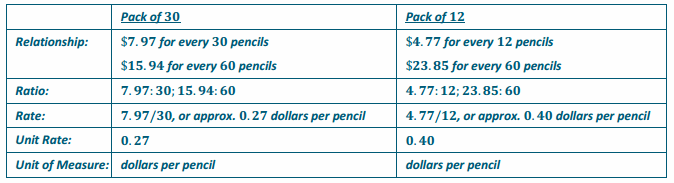
Exercise 1: Which is the Better Buy? Value-Mart is advertising a Back-to-School sale on pencils. A pack of 30 sells for $7.97, whereas a 12-pack of the same brand costs $4.77. Which is the better buy? How do you know? Answer: The better buy is the pack of 30. The pack of 30 has a smaller unit rate, approximately 0.27, as compared to the pack of 12 with a unit price of 0.40. You would pay $0.27 per pencil in the pack of 30, whereas you would pay $0.40 per pencil in the pack of 12. Students may instead choose to compare the costs for every 60 pencils or every 360 pencils, etc. Facilitate a discussion of the different methods students may have used to arrive at their decisions.
Eureka Math Grade 7 Module 1 Lesson 1 Problem Set Answer Key
Question 1. Find each rate and unit rate. a. 420 miles in 7 hours b. 360 customers in 30 days c. 40 meters in 16 seconds d. $7.96 for 5 pounds Answer: Find each rate and unit rate. a. 420 miles in 7 hours Rate: 60 miles per hour; Unit Rate: 60
b. 360 customers in 30 days Rate: 12 customers per day; Unit Rate: 12
c. 40 meters in 16 seconds Rate: \(\frac{40}{16}\), or 2.5 meters per second; Unit Rate: 2.5
$7.96 for 5 pounds Rate: \(\frac{7.96}{5}\), or approximately 1.59 dollars per pound; Unit Rate: 1.592
Question 2. Write three ratios that are equivalent to the one given: The ratio of right-handed students to left-handed students is 18:4. Answer: Sample response: The ratio of right-handed students to left-handed students is 9:2. The ratio of right-handed students to left-handed students is 36:8. The ratio of right-handed students to left-handed students is 27:6
Question 3. Mr. Rowley has 16 homework papers and 14 exit tickets to return. Ms. Rivera has 64 homework papers and 60 exit tickets to return. For each teacher, write a ratio to represent the number of homework papers to number of exit tickets they have to return. Are the ratios equivalent? Explain. Answer: Mr. Rowley’s ratio of homework papers to exit tickets is 16:14. Ms. Rivera’s ratio of homework papers to exit tickets is 64:60. The ratios are not equivalent because Mr. Rowley’s unit rate is \(\frac{8}{7}\), or approximately 1.14, and Ms. Rivera’s unit rate is \(\frac{16}{15}\), or approximately 1.07.
Question 4. Jonathan’s parents told him that for every 5 hours of homework or reading he completes, he would be able to play 3 hours of video games. His friend Lucas’s parents told their son that he could play 30 minutes for every hour of homework or reading time he completes. If both boys spend the same amount of time on homework and reading this week, which boy gets more time playing video games? How do you know? Answer: If both boys spend 5 hours on homework and reading, Jonathan will be able to play 3 hours of video games, and Lucas will be able to play 2.5 hours of video games. Jonathan gets more time playing video games. Jonathan gets 0.6 hours (36 minutes) for every 1 hour of homework and reading time, whereas Lucas gets only 30 minutes for every 1 hour of homework or reading time.
Question 5. Of the 30 girls who tried out for the lacrosse team at Euclid Middle School, 12 were selected. Of the 40 boys who tried out, 16 were selected. Are the ratios of the number of students on the team to the number of students trying out the same for both boys and girls? How do you know? Answer: Of the 30 girls who tried out for the lacrosse team at Euclid Middle School, 12 were selected. Of the 40 boys who tried out, 16 were selected. Are the ratios of the number of students on the team to the number of students trying out the same for both boys and girls? How do you know? Yes, the ratios are the same: girls—12 to 30 or 2 to 5; boys—16 to 40 or 2 to 5. The value of each ratio is \(\frac{2}{5}\).
Question 6. Devon is trying to find the unit price on a 6-pack of drinks on sale for $2.99. His sister says that at that price, each drink would cost just over $2.00. Is she correct, and how do you know? If she is not, how would Devon’s sister find the correct price? Answer: Devon’s sister is not correct. She divided the number of drinks by the cost, and to correctly find the unit price, she needs to divide the price by the number of drinks. \(\frac{2.99}{6}\), or approximately 0.50, is the correct unit price. The cost is approximately 0.50 dollars per drink.
Question 7. Each year Lizzie’s school purchases student agenda books, which are sold in the school store. This year, the school purchased 350 books at a cost of $1,137.50. If the school would like to make a profit of $1,500 to help pay for field trips and school activities, what is the least amount they can charge for each agenda book? Explain how you found your answer. Answer: The unit price per book the school paid is 3.25. To make $1,500, you would need to make a profit of 1500÷350=4.29 per book. 3.25+4.29 is the cost per book or $7.54. $7.54∙350 generates a revenue of $2,639, and $2,639 minus the initial cost of the books, $1,137.50 (expense), gives $1,501.50 of profit.
Students may need to see the video more than once. After watching the video the first time, it might be helpful for students to know that 100 meters is just a little longer than a football field (which measures 100 yards), and this record was recorded in 2009. Tillman the English bulldog covered a 100-meter stretch of a parking lot in a time of 19.678 seconds during the X Games XV in Los Angeles, California.
Watch the video clip of Tillman the English bulldog, the Guinness World Record holder for Fastest Dog on a Skateboard.
Question 1. At the conclusion of the video, your classmate takes out his or her calculator and says, “Wow that was amazing! That means the dog went about 5 meters in 1 second!” Is your classmate correct, and how do you know? Answer: Watch the video clip of Tillman the English bulldog, the Guinness World Record holder for Fastest Dog on a Skateboard. At the conclusion of the video, your classmate takes out his or her calculator and says, “Wow that was amazing! That means the dog went about 5 meters in 1 second!” Is your classmate correct, and how do you know? Yes, the classmate is correct. The dog traveled at an average rate of 100 meters in 19.678 seconds, or an associated rate of \(\frac{100}{19.678}\) meters per second, giving a unit rate of approximately 5.08.
Question 2. After seeing this video, another dog owner trained his dog, Lightning, to try to break Tillman’s skateboarding record. Lightning’s fastest recorded time was on a 75-meter stretch where it took him 15.5 seconds. Based on these data, did Lightning break Tillman’s record for fastest dog on a skateboard? Explain how you know. Answer: No, Lightning did not break Tillman’s record. Tillman traveled at an average rate of 5.08 meters per second (calculated from an associated rate of \(\frac{75}{15.5}\) meters per second), and Lightning traveled at an average rate of 4.84 meters per second (about \(\frac{1}{4}\) of a meter slower per second), making Tillman the faster skateboarder.
Engage NY Eureka Math 7th Grade Module 4 End of Module Assessment Answer Key
Eureka Math Grade 7 Module 4 End of Module Assessment Task Answer Key
DAY ONE: CALCULATOR ACTIVE You may use a calculator for this part of the assessment. Show your work to receive full credit.
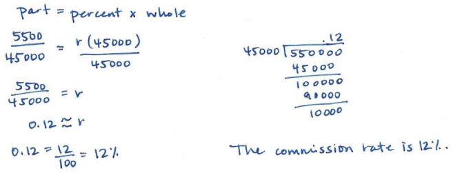
Question 1. Kara works at a fine jewelry store and earns commission on her total sales for the week. Her weekly paycheck was in the amount of $6,500, including her salary of $1,000. Her sales for the week totaled $45,000. Express her rate of commission as a percent, rounded to the nearest whole number. Answer: 6500 – 1000 = 5500 in commission r : commission rate
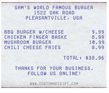
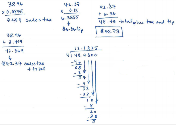
Question 2. Kacey and her three friends went out for lunch, and they wanted to leave a 15% tip. The receipt shown below lists the lunch total before tax and tip. The tip is on the cost of the food plus tax. The sales tax rate in Pleasantville is 8.75%. a. Use mental math to estimate the approximate total cost of the bill including tax and tip to the nearest dollar. Explain how you arrived at your answer. Answer: I think the bill will be about $50.00. I found my answer by rounding the total to $40.00. Then, I multiplied by 0.09, which is close to 8.75%. I got $3.60 in tax. I added that to $40.00 to get $43.60, which is close to $44.00. I know 10% of $44.00 is $440, and 5% would be $2.20. So, the total, plus a 15% tip is approximately $44.00 + $6.60 = $50.60.
b. Find the actual total of the bill including tax and tip. If Kacey and her three friends split the bill equally, how much will each person pay including tax and tip? Answer: Three people will have to pay $12.18, and one person will have to pay $12.19.
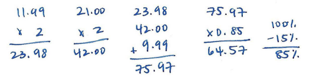
Question 3. Cool Tees is having a Back to School sale where all t-shirts are discounted by 15%. Joshua wants to buy five shirts: one costs $9.99, two cost $11.99 each, and two others cost $21.00 each. a. What is the total cost of the shirts including the discount? Answer: The total cost with the discount is $64.57.
b. By law, sales tax is calculated on the discounted price of the shirts. Would the total cost of the shirts including the 6.5% sales tax be greater if the tax was applied before a 15% discount is taken, rather than after a 15% discount is taken? Explain. Answer: The total cost would be the same because of the commutative property of multiplication. Either way, the total cost, including tax and discount, is $68.77 Tax applied after discount cost = Percent × whole × Rate Tax = (0.85) (75.97) (1.065) = 68.77
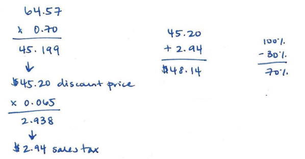
c. Joshua remembered he had a coupon in his pocket that would take an additional 30% off the price of the shirts. Calculate the new total cost of the shirts including the sales tax. Answer: The new total cost of the shirts will be $48.14.
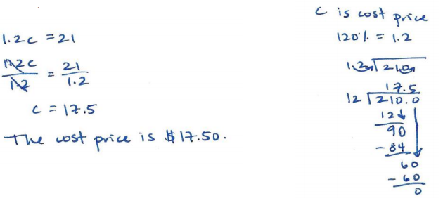
d. If the price of each shirt is 120% of the wholesale price, write an equation and find the wholesale price for a $21 shirt. Answer:
Question 4. Tierra, Cameron, and Justice wrote equations to calculate the amount of money in a savings account after one year with \(\frac{1}{2}\)% interest paid annually on a balance of M dollars. Let T represent the total amount of money saved. Tierra’s Equation: T = 1.05M Cameron’s Equation: T = M + 0.005M Justice’s Equation: T = M(1 + 0.005) a. The three students decided to see if their equations would give the same answer by using a $100 balance. Find the total amount of money in the savings account using each student’s equation. Show your work. Answer: T = 1.05($100) = $105 T = $100 + 0.005($100) = $100 + $0.5 = $100.50 T = $100(1 + 0.005) = $100(1.005) = $100.50
b. Explain why their equations will or will not give the same answer. Answer: Cameron’s and justice’s equations give the same answers but Tiara’s does not. Tiara’s equation is set up correctly, but she made a mistake when she changed \(\frac{1}{2}\)% to a decimal. \(\frac{1}{2}\)% = 0.5% = 0.005 Cameron and justice both used the distributive property to solve their equations and the correct decimal of 0.005. This is why their answers are the same.
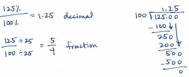
Question 5. A printing company is enlarging the image on a postcard to make a greeting card. The enlargement of the postcard’s rectangular image is done using a scale factor of 125%. Be sure to show all other related math work used to answer the following questions. a. Represent a scale factor of 125% as a fraction and decimal. Answer:
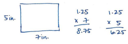
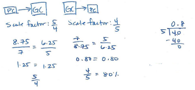
b. The postcard’s dimensions are 7 inches by 5 inches. What are the dimensions of the greeting card? Answer: The dimensions of the greeting card are 8.75 in. by 6.25 in.
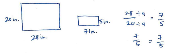
c. If the printing company makes a poster by enlarging the postcard image, and the poster’s dimensions are 28 inches by 20 inches, represent the scale factor as a percent. Answer: 4 is the scale factor, which is 400%.
d. Write an equation, in terms of the scale factor, that shows the relationship between the areas of the postcard and poster. Explain your equation. Answer: Area of Poster A = lw = (28 in)(20 in) = 560 in2
Area of Post card A = lw = (7 in) (5 in) = 35 in2 The area of the poster is 16 times the area of the post card. The scale factor is 16, or 1600%. So, my equation is P = 16c, where P is the area of the poster, 16 is the scale factor, and c is the area of the post card.
e. Suppose the printing company wanted to start with the greeting card’s image and reduce it to create the postcard’s image. What scale factor would they use? Represent this scale factor as a percent. Answer: The scale factor is 80%.
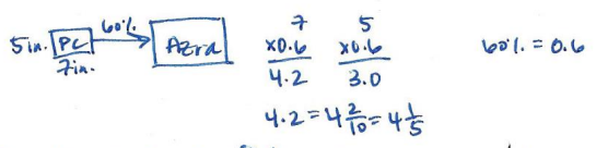
f. In math class, students had to create a scale drawing that was smaller than the postcard image. Azra used a scale factor of 60% to create the smaller image. She stated the dimensions of her smaller image as 4\(\frac{1}{6}\) inches by 3 inches. Azra’s math teacher did not give her full credit for her answer. Why? Explain Azra’s error, and write the answer correctly. Answer: Azra did not receive full credit because she made an error when changing her decimal to a fraction. She wrote 4\(\frac{2}{10}\) = 4\(\frac{1}{6}\), but it is 4\(\frac{2}{10}\) = 4\(\frac{1}{5}\) because 2 and 10 are divisible by 2. The dimensions of her image are 4\(\frac{1}{5}\) in. by 3 in.
DAY TWO: CALCULATOR INACTIVE You will now complete the remainder of the assessment without the use of a calculator.
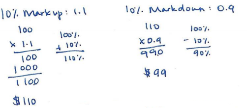
Question 6. A $100 MP3 player is marked up by 10% and then marked down by 10%. What is the final price? Explain your answer. Answer: The final price is $99.00
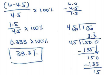
Question 7. The water level in a swimming pool increased from 4.5 feet to 6 feet. What is the percent increase in the water level rounded to the nearest tenth of a percent? Show your work. Answer:
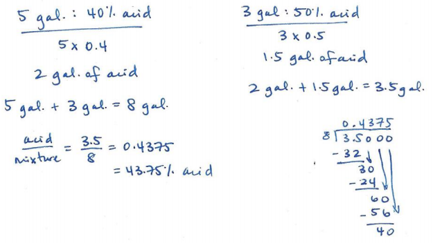
Question 8. A 5-gallon mixture contains 40% acid. A 3-gallon mixture contains 50% acid. What percent acid is obtained by putting the two mixtures together? Show your work. Answer:
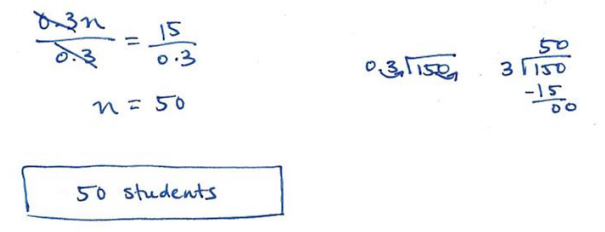
Question 9. In Mr. Johnson’s third and fourth period classes, 30% of the students scored a 95% or higher on a quiz. Let n be the total number of students in Mr. Johnson’s classes. Answer the following questions, and show your work to support your answers. a. If 15 students scored a 95% or higher, write an equation involving n that relates the number of students who scored a 95% or higher to the total number of students in Mr. Johnson’s third and fourth period classes. Answer: 0.3 n = 15
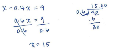
b. Solve your equation in part (a) to find how many students are in Mr. Johnson’s third and fourth period classes. Answer:
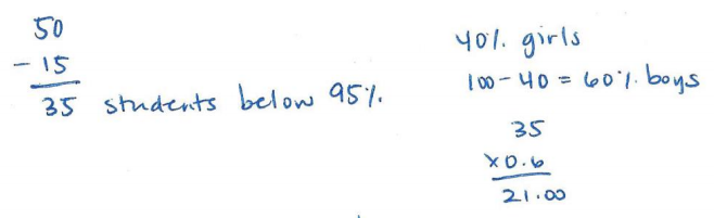
c. Of the students who scored below 95%, 40% of them are girls. How many boys scored below 95%? Answer: 21 students are boys.
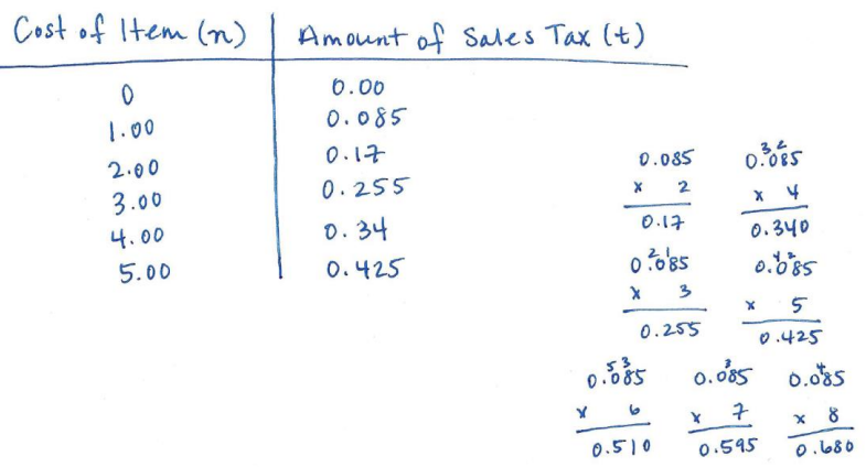
Question 1. In New York, state sales tax rates vary by county. In Allegany County, the sales tax rate is 8 1/2%. a. A book costs $12.99, and a video game costs $39.99. Rounded to the nearest cent, how much more is the tax on the video game than the tax on the book? Answer: 12.99(8.5%) = 12.99(0.085) = 1.10415 39.99(8.5%) = 39.99(0.085) = 3.39915 3.39915 – 1.10415 = 2.295 = $ 2.30
b. Using n to represent the cost of an item in dollars before tax and t to represent the amount of sales tax in dollars for that item, write an equation to show the relationship between n and t. Answer: t = 0.085 n
c. Using your equation, create a table that includes five possible pairs of solutions to the equation. Label each column appropriately. Answer:
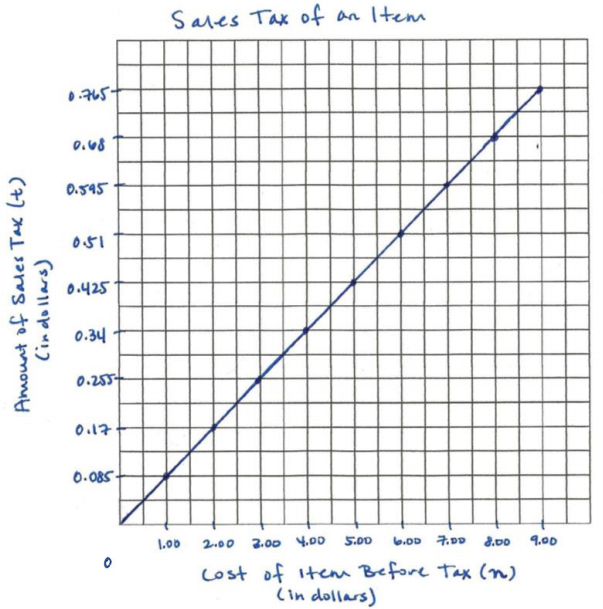
d. Graph the relationship from parts (b) and (c) in the coordinate plane. Include a title and appropriate scales and labels for both axes. Answer:
e. Is the relationship proportional? Why or why not? If so, what is the constant of proportionality? Explain. Answer: Yes, the relationship is proportional because the graph of the equation is a straight line that touches the origin. Also, the table shows that the ratio of the \(\frac{\text { amount of sales tax }}{\text { cost of an item }}\) equal 0.085. \(\frac{0.085}{1}=\frac{0.17}{2}=\frac{0.255}{3}=\frac{0.34}{4}=\frac{0.425}{5}\) The constant of proportionality is 0.085 because that is the sales tax amount for $ 1.00, which is the unit rate.
f. In nearby Wyoming County, the sales tax rate is 8%. If you were to create an equation, graph, and table for this tax rate (similar to parts (b), (c), and (d)), what would the points (0,0) and (1,0.08) represent? Explain their meaning in the context of this situation. Answer: The point of origin (0, 0) means that no tax has been applied yet because nothing has been purchased. The point (1, 0.08) is the unit rate, or the constant of proportionality. It means that for an item that costs $ 1.00, the amount of tax applied is $ 0.08. The unit rate also shows that for every 1.00, the amount of tax will increase by $ 0.08.
g. A customer returns an item to a toy store in Wyoming County. The toy store has another location in Allegany County, and the customer shops at both locations. The customer’s receipt shows $2.12 tax was charged on a $24.99 item. Was the item purchased at the Wyoming County store or the Allegany County store? Explain and justify your answer by showing your math work. Answer: The item was purchased in allegany county \(\frac{2.12}{24.99}\) is about, \(\frac{2.12}{25} \times 4\) = \(\frac{8.48}{100}\), Which is 8.48%, or about 8.5%.
Question 2. Amy is baking her famous pies to sell at the Town Fall Festival. She uses 32\(\frac{1}{2}\) cups of flour for every 10 cups of sugar in order to make a dozen pies. Answer the following questions below and show your work. a. Write an equation, in terms of f, representing the relationship between the number of cups of flour used and the number of cups of sugar used to make the pies. Answer: f = \(\frac{13}{4}\) S
b. Write the constant of proportionality as a percent. Explain what it means in the context of this situation. Answer: 3.25 = \(\frac{325}{100}\) = 3.25% A constant of proportionality of 325% means that the amount of flour used to make the pies is 325% the amount of sugar used.
c. To help sell more pies at the festival, Amy set the price for one pie at 40% less than what it would cost at her bakery. At the festival, she posts a sign that reads, “Amy’s Famous Pies—Only $9.00/Pie!” Using this information, what is the price of one pie at the bakery? Answer: The price of one pie at the bakery is $15.00.
Engage NY Eureka Math 7th Grade Module 5 Lesson 23 Answer Key
Eureka Math Grade 7 Module 5 Lesson 23 Example Answer Key
Example 1: Texting With texting becoming so popular, Linda wanted to determine if middle school students memorize real words more or less easily than fake words. For example, real words are food, car, study, swim; whereas fake words are stk, fonw, cqur, ttnsp. She randomly selected 28 students from all middle school students in her district and gave half of them a list of 20 real words and the other half a list of 20 fake words.
a. How do you think Linda might have randomly selected 28 students from all middle school students in her district? Answer: Random selection is done in an attempt to obtain students to represent all middle school students in the district. Linda would need to number all middle school students and use a random device to generate 28 numbers. One device to generate integers is http://www.rossmanchance.com/applets/RandomGen/GenRandom01.htm. Note that if there are duplicates, additional random numbers need to be generated. A second way to generate the random selections is by using the random number table provided in previous lessons.
b. Why do you think Linda selected the students for her study randomly? Explain. Answer: Linda randomly assigned her chosen 28 students to two groups of 14 each. Random assignment is done to help ensure that groups are similar to each other.
c. She gave the selected students one minute to memorize their lists, after which they were to turn the lists over and, after two minutes, write down all the words that they could remember. Afterward, they calculated the number of correct words that they were able to write down. Do you think a penalty should be given for an incorrect word written down? Explain your reasoning. Answer: Answers will vary. Either position is acceptable. The purpose is to get students to take a position and argue for it.
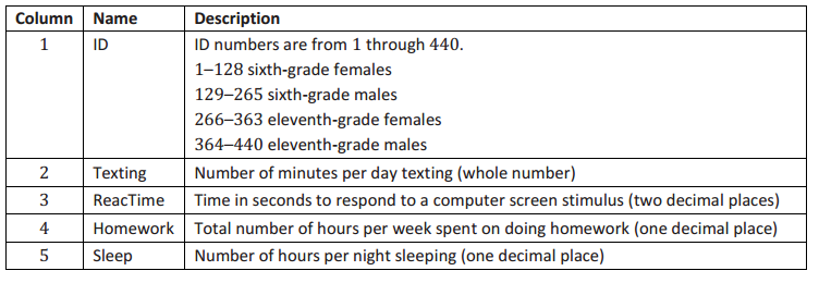
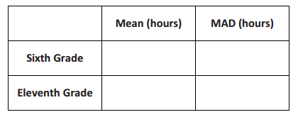
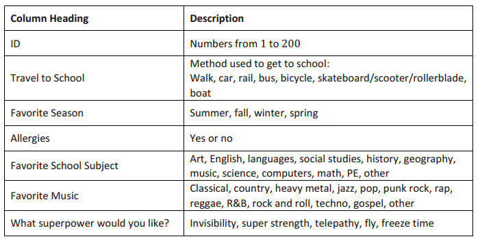
Example 2. Ken, an eighth-grade student, was interested in doing a statistics study involving sixth-grade and eleventh-grade students in his school district. He conducted a survey on four numerical variables and two categorical variables (grade level and gender). His Excel population database for the 265 sixth graders and 175 eleventh graders in his district has the following description: a. Ken decides to base his study on a random sample of 20 sixth graders and a random sample of 20 eleventh graders. The sixth graders have IDs 1–265, and the eleventh graders are numbered 266–440. Advise him on how to randomly sample 20 sixth graders and 20 eleventh graders from his data file. Answer: Ken should first number the sixth graders from 1 to 265 and the eleventh graders from 266 to 440. Then, Ken can choose 20 different random integers from 1to 265 for the sixth-grade participants and 20 different random integers from 266 to 440 for the eleventh graders.
Suppose that from a random number generator: The random ID numbers for Ken’s 20 sixth graders: 231 15 19 206 86 183 233 253 142 36 195 139 75 210 56 40 66 114 127 9 The random ID numbers for his 20 eleventh graders: 391 319 343 426 307 360 289 328 390 350 279 283 302 287 269 332 414 267 428 280
b. For each set, find the homework hours data from the population database that correspond to these randomly selected ID numbers. Answer: Sixth graders’ IDs ordered: 9 15 19 36 40 56 66 75 86 114 127 139 142 183 195 206 210 231 233 253 Their data: 8.4 7.2 9.2 7.9 9.3 7.6 6.5 6.7 8.2 7.7 7.7 4.8 5.4 4.7 7.1 6.6 2.9 8.5 6.1 8.6 Eleventh graders’ IDs ordered: 267 269 279 280 283 287 289 302 307 319 328 332 343 350 360 390 391 414 426 428 Their data: 9.5 9.8 10.9 11.8 10.0 12.0 9.1 11.8 10.0 8.3 10.6 9.5 9.8 10.8 10.7 9.4 13.2 7.3 11.6 10.3
c. On the same scale, draw dot plots for the two sample data sets. Answer:
d. From looking at the dot plots, list some observations comparing the number of hours per week that sixth graders spend on doing homework and the number of hours per week that eleventh graders spend on doing homework. Answer: There is some overlap between the data for the two random samples. The sixth-grade distribution may be slightly skewed to the left. The eleventh-grade distribution is fairly symmetric. The mean number of homework hours for sixth graders appears to be around 7 hours, whereas that for the eleventh graders is around 10.
e. Calculate the mean and MAD for each of the data sets. How many MADs separate the two sample means? (Use the larger MAD to make this calculation if the sample MADs are not the same.) Answer: The number of MADs that separate the two means is \(\frac{10.32-7.055}{1.274}\), or 2.56.
f. Ken recalled Linda suggesting that if the number of MADs is greater than or equal to 2, then it would be reasonable to think that the population of all sixth-grade students in his district and the population of all eleventh-grade students in his district have different means. What should Ken conclude based on his homework study? Answer: Since 2.56 is greater than 2, it is reasonable to conclude that on average eleventh graders spend more time doing homework per week than do sixth graders.
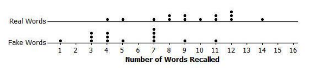
Exercises 1–4 Suppose the data (the number of correct words recalled) she collected were as follows: For students given the real words list: 8,11,12,8,4,7,9,12,12,9,14,11,5,10 For students given the fake words list: 3,5,4,4,4,7,11,9,7,7,1,3,3,7
Exercise 1. On the same scale, draw dot plots for the two data sets. Answer:
Exercise 2. From looking at the dot plots, write a few sentences comparing the distribution of the number of correctly recalled real words with the distribution of the number of correctly recalled fake words. In particular, comment on which type of word, if either, that students recall better. Explain. Answer: There is a considerable amount of overlap between data from the two random samples. The distribution of the number of real words recalled is somewhat skewed to the left; the distribution of the number of fake words recalled is fairly symmetric. The real words distribution appears to be centered around 9 or 10, whereas the fake words distribution appears to be centered around 6. Whether the separation between 9 and 6 is meaningful remains to be seen. If it is meaningful, then the mean number of real words recalled is greater than the mean number of fake words recalled.
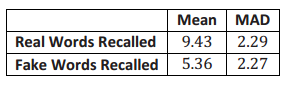
Exercise 3. Linda made the following calculations for the two data sets: In the previous lesson, you calculated the number of MADs that separated two sample means. You used the larger MAD to make this calculation if the two MADs were not the same. How many MADs separate the mean number of real words recalled and the mean number of fake words recalled for the students in the study? Answer: The difference between the two means is 9.43 – 5.36 = 4.07. The larger of the two MADs is 2.29. The number of MADs that separate the two means is \(\frac{4.07}{2.29}\), or 1.78.
Exercise 4. In the last lesson, our work suggested that if the number of MADs that separate the two sample means is 2 or more, then it is reasonable to conclude that not only do the means differ in the samples but that the means differ in the populations as well. If the number of MADs is less than 2, then you can conclude that the difference in the sample means might just be sampling variability and that there may not be a meaningful difference in the population means. Using these criteria, what can Linda conclude about the difference in population means based on the sample data that she collected? Be sure to express your conclusion in the context of this problem. Answer: Since 1.78 is below the suggested 2 MADs, Linda would conclude that the average number of real words that all middle school students in her district would recall might be the same as the average number of fake words that they would recall.
Eureka Math Grade 7 Module 5 Lesson 23 Problem Set Answer Key
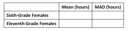
Question 1. Based on Ken’s population database, compare the amount of sleep that sixth-grade females get on average to the amount of sleep that eleventh-grade females get on average. Find the data for 15 sixth-grade females based on the following random ID numbers: 65 1 67 101 106 87 85 95 120 4 64 74 102 31 128 Find the data for 15 eleventh-grade females based on the following random ID numbers: 348 313 297 351 294 343 275 354 311 328 274 305 288 267 301 Answer: This problem compares the amount of sleep that sixth-grade females get on average to the amount of sleep that eleventh-grade females get on average. (Note to teachers: Random numbers are provided for students. Provide students access to the data file (a printed copy or access to the file at the website), or if that is not possible, provide them the following values to use in the remaining questions.) Sixth-grade females’ number of hours of sleep per night: 8.2 7.8 8.0 8.1 8.7 9.0 8.9 8.7 8.4 9.0 8.4 8.5 8.8 8.5 9.2 Eleventh-grade females’ number of hours of sleep per night: 6.9 7.8 7.2 7.9 7.8 6.7 7.6 7.3 7.7 7.3 6.5 7.7 7.2 6.3 7.5
Question 2. On the same scale, draw dot plots for the two sample data sets. Answer:
Question 3. Looking at the dot plots, list some observations comparing the number of hours per week that sixth graders spend on doing homework and the number of hours per week that eleventh graders spend on doing homework. Answer: There is a small amount of overlap between the data sets for the two random samples. The distribution of sixth-grade hours of sleep is symmetric, whereas that for eleventh graders is skewed to the left. It appears that the mean number of hours of sleep for sixth-grade females is around 8.5, and the mean number for eleventh-grade females is around 7.3 or so. Whether or not the difference is meaningful depends on the amount of variability that separates them.
Question 4. Calculate the mean and MAD for each of the data sets. How many MADs separate the two sample means? (Use the larger MAD to make this calculation if the sample MADs are not the same.) Answer: The number of MADs that separate the two means is \(\frac{8.55-7.29}{0.4}\), or 3.15.
Question 5. Recall that if the number of MADs in the difference of two sample means is greater than or equal to 2, then it would be reasonable to think that the population means are different. Using this guideline, what can you say about the average number of hours of sleep per night for all sixth-grade females in the population compared to all eleventh-grade females in the population? Answer: Since 3.15 is well above the criteria of 2 MADs, it can be concluded that on average sixth-grade females get more sleep per night than do eleventh-grade females.
Question 1. Do eleventh-grade males text more per day than eleventh-grade females do? To answer this question, two randomly selected samples were obtained from the Excel data file used in this lesson. Indicate how 20 randomly selected eleventh-grade females would be chosen for this study. Indicate how 20 randomly selected eleventh-grade males would be chosen. Answer: To pick 20 females, 20 randomly selected numbers from 266 to 363 would be generated from a random number generator or from a random number table. Duplicates would be disregarded, and a new number would be generated. To pick 20 males, 20 randomly selected numbers from 264 to 440 would be generated. Again, duplicates would be disregarded, and a new number would be generated.
Question 2. Two randomly selected samples (one of eleventh-grade females and one of eleventh-grade males) were obtained from the database. The results are indicated below: Is there a meaningful difference in the number of minutes per day that eleventh-grade females and males text? Explain your answer. Answer: The difference in the means is 02.55 min. – 100.32 min., or 2.23 min. (to the nearest hundredth of a minute). Divide this by 1.31 min. or the MAD for females (the larger of the two MADs): \(\frac{2.23}{1.31}\), or 1.70 to the nearest hundredth. This difference is less than 2 MADs, and therefore, the difference in the male and female number of minutes per day of texting is not a meaningful difference.
Engage NY Eureka Math 7th Grade Module 5 Lesson 22 Answer Key
Eureka Math Grade 7 Module 5 Lesson 22 Example Answer Key
Examples 1–3 Tamika’s mathematics project is to see whether boys or girls are faster in solving a KenKen-type puzzle. She creates a puzzle and records the following times that it took to solve the puzzle (in seconds) for a random sample of 10 boys from her school and a random sample of 11 girls from her school:
Example 1. On the same scale, draw dot plots for the boys’ data and for the girls’ data. Comment on the amount of overlap between the two dot plots. How are the dot plots the same, and how are they different? Answer: The dot plots appear to have a considerable amount of overlap. The boys’ data may be slightly skewed to the left, whereas the girls’ are relatively symmetric.
Example 2. Compare the variability in the two data sets using the MAD (mean absolute deviation). Is the variability in each sample about the same? Interpret the MAD in the context of the problem. Answer: The variability in each data set is about the same as measured by the mean absolute deviation (around 4 sec.) For boys and girls, a typical deviation from their respective mean times (35 for boys and 39 for girls) is about 4 sec.
Example 3. In the previous lesson, you learned that a difference between two sample means is considered to be meaningful if the difference is more than what you would expect to see just based on sampling variability. The difference in the sample means of the boys’ times and the girls’ times is 4.1 seconds (39.4 seconds – 35.3 seconds). This difference is approximately 1 MAD. a. If4 sec. is used to approximate the value of 1 MAD for both boys and for girls, what is the interval of times that are within 1 MAD of the sample mean for boys? Answer: 35.3 sec.+ 4 sec.=9.3 sec. , and 35.3 sec.- 4 sec.=31.4 sec. The interval of times that are within 1 MAD of the boys’ mean time is approximately 31.4 sec. to 39.3 sec.
b. Of the 10 sample means for boys, how many of them are within that interval? Answer: Six of the sample means for boys are within the interval.
c. Of the 11 sample means for girls, how many of them are within the interval you calculated in part (a)? Answer: Seven of the sample means for girls are within the interval.
d. Based on the dot plots, do you think that the difference between the two sample means is a meaningful difference? That is, are you convinced that the mean time for all girls at the school (not just this sample of girls) is different from the mean time for all boys at the school? Explain your choice based on the dot plots. Answer: Answers will vary. Sample answer: I don’t think that the difference is meaningful. The dot plots overlap a lot, and there is a lot of variability in the times for boys and the times for girls.
Examples 4–7 How good are you at estimating a minute? Work in pairs. Flip a coin to determine which person in the pair will go first. One of you puts your head down and raises your hand. When your partner says “Start,” keep your head down and your hand raised. When you think a minute is up, put your hand down. Your partner will record how much time has passed. Note that the room needs to be quiet. Switch roles, except this time you talk with your partner during the period when the person with his head down is indicating when he thinks a minute is up. Note that the room will not be quiet. Answer: Use your class data to complete the following. Example 4. Calculate the mean minute time for each group. Then, find the difference between the quiet mean and the talking mean. Answer: The mean of the quiet estimates is 58.8 sec. The mean of the talking estimates is 64.8 sec. 64.8 – 58.8 = 6 The difference between the two means is 6 sec.
Example 5. On the same scale, draw dot plots of the two data distributions, and discuss the similarities and differences in the two distributions. Answer: The dot plots have quite a bit of overlap. The quiet group distribution is fairly symmetric; the talking group distribution is skewed somewhat to the right. The variability in each is about the same. The quiet group appears to be centered around 60 sec., and the talking group appears to be centered around 65 sec.
Example 6. Calculate the mean absolute deviation (MAD) for each data set. Based on the MADs, compare the variability in each sample. Is the variability about the same? Interpret the MADs in the context of the problem. Answer: The MAD for the quiet distribution is 2.68 sec. The MAD for the talking distribution is 2.73 sec. The MAD measurements are about the same, indicating that the variability in each data set is similar. In both groups, a typical deviation of students’ minute estimates from their respective means is about 2.7 sec.
Example 7. Based on your calculations, is the difference in mean time estimates meaningful? Part of your reasoning should involve the number of MADs that separate the two sample means. Note that if the MADs differ, use the larger one in determining how many MADs separate the two means. Answer: The number of MADs that separate the two sample means is \(\frac{6}{2.73}\), or 2.2. There is a meaningful difference between the means.
Eureka Math Grade 7 Module 5 Lesson 22 Problem Set Answer Key
Question 1. A school is trying to decide which reading program to purchase. a. How many MADs separate the mean reading comprehension score for a standard program (mean = 67.8, MAD = 4.6, n = 24) and an activity-based program (mean = 70.3, MAD = 4.5, n = 27)? Answer: The number of MADs that separate the sample mean reading comprehension score for a standard program and an activity-based program is \(\frac{70.3-67.8}{4.6}\), or 0.54, about half a MAD.
b. What recommendation would you make based on this result? Answer: The number of MADs that separate the programs is not large enough to indicate that one program is better than the other program based on mean scores. There is no noticeable difference in the two programs.
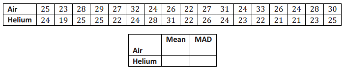
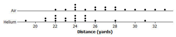
Question 2. Does a football filled with helium go farther than one filled with air? Two identical footballs were used: one filled with helium and one filled with air to the same pressure. Matt was chosen from the team to do the kicking. Matt did not know which ball he was kicking. The data (in yards) follow. Answer:
a. Calculate the difference between the sample mean distance for the football filled with air and for the one filled with helium. Answer: The 17 air-filled balls had a mean of 27 yd. compared to 23.8 yd. for the 17 helium-filled balls, a difference of 3.2 yd.
b. On the same scale, draw dot plots of the two distributions, and discuss the variability in each distribution. Answer: Based on the dot plots, it looks like the variability in the two distributions is about the same.
c. Calculate the MAD for each distribution. Based on the MADs, compare the variability in each distribution. Is the variability about the same? Interpret the MADs in the context of the problem. Answer: The MAD is 2.59 yd. for the air-filled balls and 2.07 yd. for the helium-filled balls. The typical deviation from the mean of 27.0 is about 2.59 yd. for the air-filled balls. The typical deviation from the mean of 23.8 is about 2.07 yd. for the helium-filled balls. There is a slight difference in variability.
d. Based on your calculations, is the difference in mean distance meaningful? Part of your reasoning should involve the number of MADs that separate the sample means. Note that if the MADs differ, use the larger one in determining how many MADs separate the two means. Answer: \(\frac{3.2}{2.59}\) = 1.2 There is a separation of 1.2 MADs. There is no meaningful distance between the means.
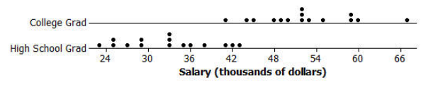
Question 3. Suppose that your classmates were debating about whether going to college is really worth it. Based on the following data of annual salaries (rounded to the nearest thousand dollars) for college graduates and high school graduates with no college experience, does it appear that going to college is indeed worth the effort? The data are from people in their second year of employment. a. Calculate the difference between the sample mean salary for college graduates and for high school graduates. Answer: The 15 college graduates had a mean salary of $52,400, compared to $32,800 for the 15 high school graduates, a difference of $19,600.
b. On the same scale, draw dot plots of the two distributions, and discuss the variability in each distribution. Answer: Based on the dot plots, the variability of the two distributions appears to be about the same.
c. Calculate the MAD for each distribution. Based on the MADs, compare the variability in each distribution. Is the variability about the same? Interpret the MADs in the context of the problem. Answer: The MAD is 5.15 for college graduates and 5.17 for high school graduates. The typical deviation from the mean of 52.4 is about 5.15 (or $5,150) for college graduates. The typical deviation from the mean of 32.8 is about 5.17 ($5,170) for high school graduates. The variability in the two distributions is nearly the same.
d. Based on your calculations, is going to college worth the effort? Part of your reasoning should involve the number of MADs that separate the sample means. Answer: \(\frac{19.6}{5.17}\) = 3.79 There is a separation of 3.79 MADs. There is a meaningful difference between the population means. Going to college is worth the effort.
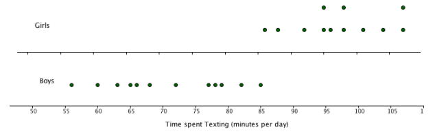
Suppose that Brett randomly sampled 12 tenth-grade girls and boys in his school district and asked them for the number of minutes per day that they text. The data and summary measures follow. Question 1. Draw dot plots for the two data sets using the same numerical scales. Discuss the amount of overlap between the two dot plots that you drew and what it may mean in the context of the problem. Answer: There is no overlap between the two data sets. This indicates that the sample means probably differ, with girls texting more than boys on average. The girls’ data set is a little more compact than the boys, indicating that their measure of variability is smaller.
Question 2. Compare the variability in the two data sets using the MAD. Interpret the result in the context of the problem. Answer: The MAD for the boys’ number of minutes spent texting is 7.9 min., which is higher than that for the girls, which is 5.3 min. This is not surprising, as seen in the dot plots. The typical deviation from the mean of 70.9 is about 7.9 min. for boys. The typical deviation from the mean of 97.3 is about 5.3 min. for girls.
Question 3. From 1 and 2, does the difference in the two means appear to be meaningful? Answer: 97.3 – 70.9 = 26.4 The difference in means is 26.4 min. \(\frac{26.4}{7.9}\) = 3.3 Using the larger MAD of 7.9 min., the means are separated by 3.3 MADs. Looking at the dot plots, it certainly seems as though a separation of more than 3 MADs is meaningful.
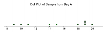
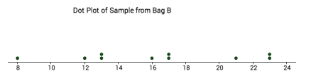
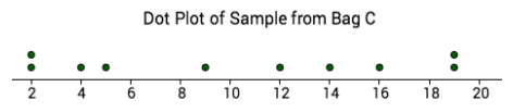
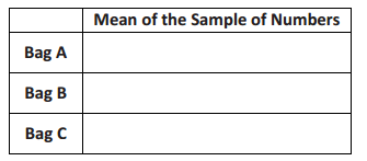
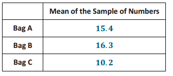
Exercise 1. To begin your investigation, start by selecting a random sample of ten numbers from Bag A. Remember to mix the numbers in the bag first. Then, select one number from the bag. Do not put it back into the bag. Write the number in the chart below. Continue selecting one number at a time until you have selected ten numbers. Mix up the numbers in the bag between each selection. Answer:
a. Create a dot plot of your sample of ten numbers. Use a dot to represent each number in the sample. Answer: The dot plot will vary based on the sample selected. One possible answer is shown here.
b. Do you think the mean of all the numbers in Bag A might be 10? Why or why not? Answer: Anticipate that students will indicate a mean of a sample from Bag A is greater than 10. Responses depend on students’ samples and the resulting dot plots. In most cases, the dots will center around a value that is greater than 10 because the mean of the population is greater than 10.
c. Based on the dot plot, what would you estimate the mean of the numbers in Bag A to be? How did you make your estimate? Answer: Answers will vary depending on students’ samples. Anticipate that most students’ estimates will correspond to roughly where the dots in the dot plot center. The population mean here is 14.5, so answers around 14 or 15 would be expected.
d. Do you think your sample mean will be close to the population mean? Why or why not? Answer: Students could answer “Yes,” “No,” or “I don’t know.” The goal of this question is to get students to think about the difference between a sample mean and the population mean.
e. Is your sample mean the same as your neighbors’ sample means? Why or why not? Answer: No. When selecting a sample at random, different students get different sets of numbers. This is sampling variability.
Exercise 2. Repeat the process by selecting a random sample of ten numbers from Bag B. Answer:
a. Create a dot plot of your sample of ten numbers. Use a dot to represent each of the numbers in the sample. Answer: The dot plots will vary based on the sample selected. One possible answer is shown here.
b. Based on your dot plot, do you think the mean of the numbers in Bag C is the same as or different from the mean of the numbers in Bag A? Explain your thinking. Answer: Answers will vary, as students will compare their center of the dot plot of the sample from Bag B to the center of the dot plot of the sample from Bag A. The centers will probably not be exactly the same; however, anticipate centers that are close to each other.
Exercise 3. Repeat the process once more by selecting a random sample of ten numbers from Bag C. Answer:
a. Create a dot plot of your sample of ten numbers. Use a dot to represent each of the numbers in the sample. Answer: The dot plots will vary based on the sample selected. One possible answer is shown here.
b. Based on your dot plot, do you think the mean of the numbers in Bag C is the same as or different from the mean of the numbers in Bag A? Explain your thinking. Answer: Anticipate that students will indicate that the center of the dot plot of the sample from Bag C is less than the center of the dot plot of the sample from Bag A. Because the population mean for Bag C is less than the population mean for Bag A, the center of the dot plot will usually be less for the sample from Bag C.
Exercise 4. Are your dot plots of the three bags the same as the dot plots of other students in your class? Why or why not? Answer: The dot plots will vary. Because different students generally get different samples when they select a sample from the bags, the dot plots will vary from student to student.
Exercise 5. Calculate the mean of the numbers for each of the samples from Bag A, Bag B, and Bag C. Answer:
a. Are the sample means you calculated the same as the sample means of other members of your class? Why or why not? Answer: No. When selecting a sample at random, you get different sets of numbers (again, sampling variability).
b. How do your sample means for Bag A and for Bag B compare? Answer: Students might answer that the mean for the sample from Bag A is larger, smaller, or equal to the mean for the sample from Bag B, depending on their samples. For the example given above, the sample mean for Bag A is smaller than the sample mean for Bag B.
c. Calculate the difference of the sample mean for Bag A minus the sample mean for Bag B (Mean A – Mean B). Based on this difference, can you be sure which bag has the larger population mean? Why or why not? Answer: No. It is possible that you could get a sample mean that is larger than the population mean of Bag A and then get a sample mean that is smaller than the population mean of Bag B, or vice versa.
Exercise 6. Based on the class dot plots of the sample means, do you think the mean of the numbers in Bag A and the mean of the numbers in Bag B are different? Do you think the mean of the numbers in Bag A and the mean of the numbers in Bag C are different? Explain your answers. Answer: Answers will vary. Sample response: Bags A and B are similar, and Bag C is different from the other two.
Exercise 7. Based on the difference between the sample mean of Bag A and the sample mean of Bag B (Mean A – Mean B) that you calculated in Exercise 5, do you think that the two populations (Bags A and B) have different means, or do you think that the two population means might be the same? Answer: Answers will vary, as the difference of the means will be based on each student’s samples. Anticipate answers that indicate the difference in the sample means that the population means might be the same for differences that are close to 0. (Students learn later in this lesson that the populations of Bags A and B are the same, so most students will see differences that are not too far from 0.)
Exercise 8. Based on this difference, can you be sure which bag has the larger population mean? Why or why not? Answer: No. It is possible that you could get a sample mean that is larger than the population mean of Bag A and then get a sample mean that is smaller than the population mean of Bag B, or vice versa.
Exercise 9. Is your difference in sample means the same as your neighbors’ differences? Why or why not? Answer: No. As the samples will vary due to sampling variability, so will the means of each sample.
Exercise 10. Plot your difference of the means (Mean A – Mean B) on a class dot plot. Describe the distribution of differences plotted on the graph. Remember to discuss center and spread. Answer: Answers will vary. The distribution of the differences is expected to cluster around 0. One example for a class of 30 students is shown here.
Exercise 11. Why are the differences in the sample means of Bag A and Bag B not always 0? Answer: For the difference in sample means to be 0, the sample means must be the same value. This would rarely happen when selecting random samples.
Exercise 12. Does the class dot plot contain differences that were relatively far away from 0? If yes, why do you think this happened? Answer: For the dot plot given as an example above, some differences were as large as 4.
Exercise 13. Suppose you will take a sample from a new bag. How big would the difference in the sample mean for Bag A and the sample mean for the new bag (Mean A – Mean new) have to be before you would be convinced that the population mean for the new bag is different from the population mean of Bag A? Use the class dot plot of the differences in sample means for Bags A and B (which have equal population means) to help you answer this question. Answer: Students should recognize that the difference would need to be relatively far away from 0. They may give answers like “a difference of 5 (or larger)” or something similar. Remind students that the differences noted in the class dot plot are a result of sampling from bags that have the same numbers in them. As a result, students would be expected to suggest values that are greater than the values in the class dot plot.
Exercise 14. Calculate the sample mean of Bag A minus the sample mean of Bag C (Mean A – Mean C). Answer: Answers will vary, as the samples collected by students will vary. Students might suspect, however, that they are being set up for a discussion about populations that have different means. As a result, ask students what they think their difference is indicating about the populations of the two bags. For several students, this difference is larger than the difference they received for Bags A and B and might suggest that the means of the bags are different.
Not all students, however, will have differences that are noticeably different from what they obtained for Bags A and B, and as a result, they will indicate that the bags could have the same or similar distribution of numbers.
Exercise 15. Plot your difference (Mean A – Mean C) on a class dot plot. Answer: Have each student or group of students place their differences on a class dot plot similar to what was developed for the dot plot of the difference of means in Bags A and B. Place the dot plots next to each other so that students can compare the centers and spread of each distribution. One example based on a class of 30 students is shown here. Notice that the differences for Bag A – Bag B center around 0, while the differences for Bag A – Bag C do not center around 0.
Exercise 16. How do the centers of the class dot plots for Mean A – Mean B and Mean A – Mean C compare? Answer: The center of the second dot plot Mean A – Mean C is shifted over to the right. Thus, it is not centered at 0; rather, it is centered over a value that is larger than 0.
Exercise 17. Each bag has a population mean that is either 10.5 or 14.5. State what you think the population mean is for each bag. Explain your choice for each bag. Answer: The population mean is 14.5 for Bags A and B and 10.5 for Bag C. Students indicate their selections based on the class dot plots and the sample means they calculated in the exercises.
Eureka Math Grade 7 Module 5 Lesson 21 Problem Set Answer Key
Below are three dot plots. Each dot plot represents the differences in sample means for random samples selected from two populations (Bag A and Bag B). For each distribution, the differences were found by subtracting the sample means of Bag B from the sample means of Bag A (sample mean A – sample mean B). Question 1. Does the graph below indicate that the population mean of Bag A is larger than the population mean of Bag B? Why or why not? Answer: No. Since most of the differences are negative, it appears that the population mean of Bag A is smaller than the population mean of Bag B.
Question 2. Use the graph above to estimate the difference in the population means (Mean A – Mean B). Answer: About -4. This is about the middle of the graph.
Question 3. Does the graph below indicate that the population mean of Bag A is larger than the population mean of Bag B? Why or why not? Answer: No. The dots are all centered around 0, meaning that the population means of Bag A and Bag B might be equal.
Question 4. Does the graph below indicate that the population mean of Bag A is larger than the population mean of Bag B? Why or why not? Answer: Yes. The dots are near 1.5. There is a small difference in the population means, but it is so small that it is difficult to detect. (Note to teachers: Some students may answer, “No. The dots appear centered around 0.” Problem 6 should cause students to rethink this answer.)
Question 5. In the above graph, how many differences are greater than 0? How many differences are less than 0? What might this tell you? Answer: There are 18 dots greater than 0 and 12 dots less than 0. It tells me that there are more positive differences, which may mean that the population mean for Bag A is bigger than the population mean for Bag B.
Question 6. In Problem 4, the population mean for Bag A is really larger than the population mean for Bag B. Why is it possible to still get so many negative differences in the graph? Answer: It is possible to get so many negative values because the population mean of Bag A may only be a little bigger than the population mean of Bag B.
Question 1. How is a meaningful difference in sample means different from a non-meaningful difference in sample means? You may use what you saw in the dot plots of this lesson to help you answer this question. Answer: A meaningful difference in sample means is one that is not likely to have occurred by just chance if there is no difference in the population means. A meaningful difference in sample means would be one that is very far from 0 (or not likely to happen if the population means are equal). A non-meaningful difference in sample means would be one that is relatively close to 0, which indicates the population means are equal.
Note that how big this difference needs to be in order to be declared meaningful depends on the context, the sample size, and the variability in the populations.
Engage NY Eureka Math 7th Grade Module 5 Lesson 20 Answer Key
Eureka Math Grade 7 Module 5 Lesson 20 Example Answer Key
Example 2: Estimating Population Proportion Two hundred middle school students at Roosevelt Middle School responded to several survey questions. A printed copy of the responses the students gave to various questions will be provided by your teacher. The data are organized in columns and are summarized by the following table: The last column in the data file is based on the question: Which of the following superpowers would you most like to have? The choices were invisibility, super strength, telepathy, fly, or freeze time.
The class wants to determine the proportion of Roosevelt Middle School students who answered “freeze time” to the last question. You will use a sample of the Roosevelt Middle School population to estimate the proportion of the students who answered “freeze time” to the last question. A random sample of 20 student responses is needed. You are provided the random number table you used in a previous lesson. A printed list of the 200 Roosevelt Middle School students is also provided. In small groups, complete the following exercise: a. Select a random sample of 20 student responses from the data file. Explain how you selected the random sample. Answer: Generate 20 random numbers between 1 and 200. The random number chosen represents the ID number of the student. Go to that ID number row, and record the outcome as “yes” or “no” in the table regarding the freeze time response.
b. In the table below, list the 20 responses for your sample. Answer: Answers will vary. Below is one possible result.
c. Estimate the population proportion of students who responded “freeze time” by calculating the sample proportion of the 20 sampled students who responded “freeze time” to the question. Answer: Students’ answers will vary. The sample proportion in the given example is \(\frac{5}{20}\), or 0.25.
d. Combine your sample proportion with other students’ sample proportions, and create a dot plot of the distribution of the sample proportions of students who responded “freeze time” to the question. Answer: An example is shown below. The class dot plot may differ somewhat from the one below, but the distribution should center at approximately 0.20. (Provide students this distribution of sample proportions if they were unable to obtain a distribution.)
e. By looking at the dot plot, what is the value of the proportion of the 200 Roosevelt Middle School students who responded “freeze time” to the question? Answer: 0.20
f. Usually, you will estimate the proportion of Roosevelt Middle School students using just a single sample proportion. How different was your sample proportion from your estimate based on the dot plot of many samples? Answer: Students’ answers will vary depending on their sample proportions. For this example, the sample proportion is 0.25, which is slightly greater than the 0.20.
g. Circle your sample proportion on the dot plot. How does your sample proportion compare with the mean of all the sample proportions? Answer: The mean of the class distribution will vary from this example. The class distribution should center at approximately 0.20.
h. Calculate the mean of all of the sample proportions. Locate the mean of the sample proportions in your dot plot; mark this position with an X. How does the mean of the sample proportions compare with your sample proportion? Answer: Answers will vary based on the samples generated by students.
Exercise 1. The first student reported a sample proportion of 0.15. Interpret this value in terms of the summary of the problem in the example. Answer: Three of the 20 students surveyed responded that they were vegetarian.
Exercise 2. Another student reported a sample proportion of 0. Did this student do something wrong when selecting the sample of middle school students? Answer: No. This means that none of the 20 students surveyed said that they were vegetarian.
Exercise 3. Assume you were part of this seventh-grade class and you got a sample proportion of 0.20 from a random sample of middle school students. Based on this sample proportion, what is your estimate for the proportion of all middle school students who are vegetarians? Answer: My estimate is 0.20.
Exercise 4. Construct a dot plot of the 30 sample proportions. Answer:
Exercise 5. Describe the shape of the distribution. Answer: Nearly symmetrical or mound shaped centering at approximately 0.15
Exercise 6. Using the 30 class results listed above, what is your estimate for the proportion of all middle school students who are vegetarians? Explain how you made this estimate. Answer: About 0.15. I chose this value because the sample proportions tend to cluster between 0.10 and 0.15 or 0.10 and 0.20.
Exercise 7. Calculate the mean of the 30 sample proportions. How close is this value to the estimate you made in Exercise 6? Answer: The mean of the 30 samples to the nearest thousandth is 0.153. The value is close to my estimate of 0.15, and if calculated to the nearest hundredth, they would be the same. (Most likely, students will say between 0.10 and 0.15.)
Exercise 8. The proportion of all middle school students who are vegetarians is 0.15. This is the actual proportion for the entire population of middle school students used to select the samples. How the mean of the 30 sample proportions compares with the actual population proportion depends on the students’ samples. Answer: In this case, the mean of the 30 sample proportions is very close to the actual population proportion.
Exercise 9. Do the sample proportions in the dot plot tend to cluster around the value of the population proportion? Are any of the sample proportions far away from 0.15? List the proportions that are far away from 0.15. Answer: They cluster around 0.15. The values of 0 and 0.30 are far away from 0.15.
Eureka Math Grade 7 Module 5 Lesson 20 Problem Set Answer Key
Question 1. A class of 30 seventh graders wanted to estimate the proportion of middle school students who played a musical instrument. Each seventh grader took a random sample of 25 middle school students and asked each student whether or not he or she played a musical instrument. The following are the sample proportions the seventh graders found in 30 samples. a. The first student reported a sample proportion of 0.80. What does this value mean in terms of this scenario? Answer: A sample proportion of 0.80 means 20 out of 25 answered yes to the survey.
b. Construct a dot plot of the 30 sample proportions. Answer:
c. Describe the shape of the distribution. Answer: Nearly symmetrical. It centers at approximately 0.72.
d. Describe the variability of the distribution. Answer: The spread of the distribution is from 0.60 to 0.84.
e. Using the 30 class sample proportions listed on the previous page, what is your estimate for the proportion of all middle school students who played a musical instrument? Answer: The mean of the 30 sample proportions is approximately 0.713.
Question 2. Select another variable or column from the data file that is of interest. Take a random sample of 30 students from the list, and record the response to your variable of interest of each of the 30 students. a. Based on your random sample, what is your estimate for the proportion of all middle school students? Answer: Students’ answers will vary depending on the column chosen.
b. If you selected a second random sample of 30, would you get the same sample proportion for the second random sample that you got for the first random sample? Explain why or why not. Answer: No. It is very unlikely that you would get exactly the same result. This is sampling variability—the value of a sample statistic will vary from one sample to another.
Thirty seventh graders each took a random sample of 10 middle school students and asked each student whether or not he likes pop music. Then, they calculated the proportion of students who like pop music for each sample. The dot plot below shows the distribution of the sample proportions. Question 1. There are three dots above 0.2. What does each dot represent in terms of this scenario? Answer: Each dot represents the survey results from one student. 0.2 means two students out of 10 said they like pop music.
Question 2. Based on the dot plot, do you think the proportion of the middle school students at this school who like pop music is 0.6? Explain why or why not. Answer: No. Based on the dot plot, 0.6 is not a likely proportion. The dots cluster at 0.3 to 0.5, and only a few dots were located at 0.6. An estimate of the proportion of students at this school who like pop music would be within the cluster of 0.3 to 0.5.
Engage NY Eureka Math 7th Grade Module 5 Lesson 19 Answer Key
Eureka Math Grade 7 Module 5 Lesson 19 Example Answer Key
Example 1: Sample Proportion Your teacher will give your group a bag that contains colored cubes, some of which are red. With your classmates, you are going to build a distribution of sample proportions. a. Each person in your group should randomly select a sample of 10 cubes from the bag. Record the data for your sample in the table below. Answer: Students’ tables will vary based on their samples.
b. What is the proportion of red cubes in your sample of 10? This value is called the sample proportion. The sample proportion is found by dividing the number of successes (in this example, the number of red cubes) by the total number of observations in the sample. Answer: Students’ results will be around 0.4. In this example, the sample proportion is 0.3.
c. Write your sample proportion on a sticky note, and place it on the number line that your teacher has drawn on the board. Place your note above the value on the number line that corresponds to your sample proportion. The graph of all students’ sample proportions is called a sampling distribution of the sample proportions. Answer: This is an example of a dot plot of the sampling distribution.
d. Describe the shape of the distribution. Answer: A nearly symmetrical distribution that is clustered around 0.4
e. Describe the variability in the sample proportions. Answer: The spread of the data is from 0.1 to 0.7. Much of the data cluster between 0.3 and 0.5.
Based on the distribution, answer the following: f. What do you think is the population proportion? Answer: Based on the dot plot, an estimate of the population proportion is approximately 0.4.
g. How confident are you of your estimate? Answer: Because there is a lot of variability from sample to sample (0.1 to 0.7), I do not have a lot of confidence in my estimate.
Example 2: Sampling Variability What do you think would happen to the sampling distribution if everyone in class took a random sample of 30 cubes from the bag? To help answer this question, you will repeat the random sampling you did in part (a) of Example 1, except now you will draw a random sample of 30 cubes instead of 10. a. Take a random sample of 30 cubes from the bag. Carefully record the outcome of each draw. Answer: Answers will vary. An example follows:
b. What is the proportion of red cubes in your sample of 30? Answer: Answers will vary. In this example, the sample proportion is \(\frac{11}{30}\), or approximately 0.367.
c. Write your sample proportion on a sticky note, and place the note on the number line that your teacher has drawn on the board. Place your note above the value on the number line that corresponds to your sample proportion. Answer: An example of a dot plot:
d. Describe the shape of the distribution. Answer: Mound shaped, centered around 0.4
Exercise 1. Describe the variability in the sample proportions. Answer: The spread of the data is from 0.25 to 0.55. Most of the data cluster between 0.35 and 0.5.
Exercise 2. Based on the distribution, answer the following: a. What do you think is the population proportion? Answer: Based on the dot plot, an estimate of the population proportion is approximately 0.4.
b. How confident are you of your estimate? Answer: Because there is less variability from sample to sample (0.35 to 0.5), I am more confident in my estimate.
c. If you were taking a random sample of 30 cubes and determined the proportion that was red, do you think your sample proportion will be within 0.05 of the population proportion? Explain. Answer: Answers depend on the dot plots prepared by students. If the dot plot in Example 2 part (c), is used as an example, note that only about half of the dots are between 0.35 and 0.45. There are several samples that had sample proportions that were farther away from the center than 0.05, so the sample proportion might not be within 0.05 of the population proportion.
Exercise 3. Compare the sampling distribution based on samples of size 10 to the sampling distribution based on samples of size 30. Answer: Both distributions are mound shaped and center around 0.4. Variability is less in the sampling distribution of sample sizes of 30 versus sample sizes of 10.
Exercise 4. As the sample size increased from 10 to 30, describe what happened to the sampling variability of the sample proportions. Answer: The sampling variability decreased as the sample size increased.
Exercise 5. What do you think would happen to the sampling variability of the sample proportions if the sample size for each sample was 50 instead of 30? Explain. Answer: The sampling variability in the sampling distribution for samples of size 50 will be less than the sampling variability of the sampling distribution for samples of size 30.
Eureka Math Grade 7 Module 5 Lesson 19 Problem Set Answer Key
Question 1. A class of seventh graders wanted to find the proportion of M&M’s® that are red. Each seventh grader took a random sample of 20 M&M’s® from a very large container of M&M’s®. The following is the proportion of red M&M’s each student found. a. Construct a dot plot of the sample proportions. Answer:
b. Describe the shape of the distribution. Answer: Somewhat mound shaped, slightly skewed to the right
c. Describe the variability of the distribution. Answer: The spread of the data is from 0.0 to 0.3. Most of the data cluster between 0.10 and 0.20.
d. Suppose the seventh-grade students had taken random samples of size 50. Describe how the sampling distribution would change from the one you constructed in part (a). Answer: The sampling variability would decrease.
Question 2. A group of seventh graders wanted to estimate the proportion of middle school students who suffer from allergies. The members of one group of seventh graders each took a random sample of 10 middle school students, and the members of another group of seventh graders each took a random sample of 40 middle school students. Below are two sampling distributions of the sample proportions of middle school students who said that they suffer from allergies. Which dot plot is based on random samples of size 40? How can you tell? Answer: Dot Plot A is based on random samples of size 40 rather than random samples of size 10 because the variability of the distribution is less than the variability in Dot Plot B.
Question 3. The nurse in your school district would like to study the proportion of middle school students who usually get at least eight hours of sleep on school nights. Suppose each student in your class plans on taking a random sample of 20 middle school students from your district, and each calculates a sample proportion of students who said that they usually get at least eight hours of sleep on school nights.
a. Do you expect everyone in your class to get the same value for their sample proportions? Explain. Answer: No. We expect sample variability.
b. Suppose each student in class increased the sample size from 20 to 40. Describe how you could reduce the sampling variability. Answer: I could reduce the sampling variability by using the larger sample size.
A group of seventh graders took repeated samples of size 20 from a bag of colored cubes. The dot plot below shows the sampling distribution of the sample proportion of blue cubes in the bag. Question 1. Describe the shape of the distribution. Answer: Mound shaped, centered around 0.55
Question 2. Describe the variability of the distribution. Answer: The spread of the data is from 0.35 to 0.75, with much of the data between 0.50 and 0.65.
Question 3. Predict how the dot plot would look differently if the sample sizes had been 40 instead of 20. Answer: The variability will decrease as the sample size increases. The dot plot will be centered in a similar place but will be less spread out.
Engage NY Eureka Math 7th Grade Module 5 Lesson 18 Answer Key
Eureka Math Grade 7 Module 5 Lesson 18 Example Answer Key
Example 1: Sampling Variability The previous lesson investigated the statistical question “What is the typical time spent at the gym?” by selecting random samples from the population of 800 gym members. Two different dot plots of sample means calculated from random samples from the population are displayed below. The first dot plot represents the means of 20 samples with each sample having 5 data points. The second dot plot represents the means of 20 samples with each sample having 15 data points. Based on the first dot plot, Jill answered the statistical question by indicating the mean time people spent at the gym was between 34 and 78 minutes. She decided that a time approximately in the middle of that interval would be her estimate of the mean time the 800 people spent at the gym. She estimated 52 minutes. Scott answered the question using the second dot plot. He indicated that the mean time people spent at the gym was between 41 and 65 minutes. He also selected a time of 52 minutes to answer the question.
a. Describe the differences in the two dot plots. Answer: The first dot plot shows a greater variability in the sample means than the second dot plot.
b. Which dot plot do you feel more confident in using to answer the statistical question? Explain your answer. Answer: Possible response: The second dot plot gives me more confidence because the sample means do not differ as much from one another. They are more tightly clustered, so I think I have a better idea of where the population mean is located.
c. In general, do you want sampling variability to be large or small? Explain. Answer: The larger the sampling variability, the more that the value of a sample statistic varies from one sample to another and the farther you can expect a sample statistic value to be from the population characteristic. You want the value of the sample statistic to be close to the population characteristic. So, you want sampling variability to be small.
Exercises 1–3 In the previous lesson, you saw a population of 800 times spent at the gym. You will now select a random sample of size 15 from that population. You will then calculate the sample mean.
Exercise 1. Start by selecting a three-digit number from the table of random digits. Place the random digit table in front of you. Without looking at the page, place the eraser end of your pencil somewhere on the table of random digits. Start using the table of random digits at the digit closest to your eraser. This digit and the following two specify which observation from the population will be the first observation in your sample. Write the value of this observation in the space below. (Discard any three-digit number that is 800 or larger, and use the next three digits from the random digit table.) Answer: Answers will vary.
Exercise 2. Continue moving to the right in the table of random digits from the point that you reached in Exercise 1. Each three-digit number specifies a value to be selected from the population. Continue in this way until you have selected 14 more values from the population. This will make 15 values altogether. Write the values of all 15 observations in the space below. Answer: Answers will vary.
Exercise 3. Calculate the mean of your 15 sample values. Write the value of your sample mean below. Round your answer to the nearest tenth. (Be sure to show your work.) Answer: Answers will vary.
Exercises 4–6 You will now use the sample means from Exercise 3 for the entire class to make a dot plot.
Exercise 4. Write the sample means for everyone in the class in the space below. Answer: Answers will vary.
Exercise 5. Use all the sample means to make a dot plot using the axis given below. (Remember, if you have repeated values or values close to each other, stack the dots one above the other.) Answer: Answers will vary.
Exercise 6. In the previous lesson, you drew a dot plot of sample means for samples of size 5. How does the dot plot above (of sample means for samples of size 15) compare to the dot plot of sample means for samples of size 5? For which sample size (5 or 15) does the sample mean have the greater sampling variability?
This exercise illustrates the notion that the greater the sample size, the smaller the sampling variability of the sample mean. Answer: The dot plots will vary depending on the results of the random sampling. Dot plots for one set of sample means for 20 random samples of size 5 and for 20 random samples of size 15 are shown below. The main thing for students to notice is that there is less variability from sample to sample for the larger sample size. This exercise illustrates the notion that the greater the sample size, the smaller the sampling variability of the sample mean.
Exercises 7–8
Exercise 7. Remember that in practice you only take one sample. Suppose that a statistician plans to take a random sample of size 15 from the population of times spent at the gym and will use the sample mean as an estimate of the population mean. Based on the dot plot of sample means that your class collected from the population, approximately how far can the statistician expect the sample mean to be from the population mean? (The actual population mean is 53.9 minutes.) Answer: Answers will vary according to the degree of variability that appears in the dot plot and a student’s estimate of an average distance from the population mean. Allow students to use an approximation of 54 minutes for the population mean. In the example above, the 20 samples could be used to estimate the mean distance of the sample means to the population mean of 54 minutes. The sum of the distances from the mean in the above example is 137. The mean of these distances, or the expected distance of a sample mean from the population mean, is 6.85 minutes.
Exercise 8. How would your answer in Exercise 7 compare to the equivalent mean of the distances for a sample of size 5? Answer: Sample response: My answer for Exercise 7 is smaller than the expected distance for the samples of size 5. For samples of size 5, several dots are farther from the mean of 54 minutes. The mean of the distance for samples of size 5 would be larger.
Exercises 9–11 Suppose everyone in your class selected a random sample of size 25 from the population of times spent at the gym.
Exercise 9. What do you think the dot plot of the class’s sample means would look like? Make a sketch using the axis below. Answer: Students’ sketches should show dots that have less spread than those in the dot plot for samples of size 15. For example, students’ dot plots might look like this:
Exercise 10. Suppose that a statistician plans to estimate the population mean using a sample of size 25. According to your sketch, approximately how far can the statistician expect the sample mean to be from the population mean? Answer: We were told in Exercise 7 that the population mean is 53.9. If you calculate the mean of the distances from the population mean (in the same way you did in Exercise 7), the average or expected distance of a sample mean from 53.9 is approximately 3 minutes for a dot plot similar to the one above. This estimate is made by approximating the average distance of each dot from 53.9 or 54. Note: If necessary, make a chart similar to what was suggested in Exercise 7. Using the dot plot, direct students to estimate the distance of each dot from 54 (rounding to the nearest whole number is adequate for this question), add up the distances, and divide by the number of dots.
Exercise 11. Suppose you have a choice of using a sample of size 5, 15, or 25. Which of the three makes the sampling variability of the sample mean the smallest? Why would you choose the sample size that makes the sampling variability of the sample mean as small as possible? Answer: Choosing a sample size of 25 makes the sampling variability of the sample mean the smallest, which is preferable because the sample mean is then more likely to be closer to the population mean than it would be for the smaller sample sizes.
Eureka Math Grade 7 Module 5 Lesson 18 Problem Set Answer Key
Question 1. The owner of a new coffee shop is keeping track of how much each customer spends (in dollars). One hundred of these amounts are shown in the table below. These amounts will form the population for this question. a. Place the table of random digits in front of you. Select a starting point without looking at the page. Then, taking two digits at a time, select a random sample of size 10 from the population above. Write the 10 values in the space below. (For example, suppose you start at the third digit of row four of the random digit table. Taking two digits gives you 19. In the population above, go to the row labeled 1, and move across to the column labeled 9. This observation is 4.98, and that will be the first observation in your sample. Then, continue in the random digit table from the point you reached.) Answer: a. For example (starting in the random digit table at the 8 th digit in row 15): 5.12, 5.47, 5.71, 6.18, 4.55, 5.12, 3.63, 5.12, 5.71, 4.34. Calculate the mean for your sample, showing your work. Round your answer to the nearest thousandth. \(\frac{5.12+5.47+5.71+6.18+4.55+5.12+3.63+5.12+5.71+4.34}{10}\) = 5.095 Calculate the mean for your sample, showing your work. Round your answer to the nearest thousandth. Answer: For example (starting in the random digit table at the 8 th digit in row 15): 5.12, 5.47, 5.71, 6.18, 4.55, 5.12, 3.63, 5.12, 5.71, 4.34. Calculate the mean for your sample, showing your work. Round your answer to the nearest thousandth. \(\frac{5.12+5.47+5.71+6.18+4.55+5.12+3.63+5.12+5.71+4.34}{10}\) = 5.095
b. Using the same approach as in part (a), select a random sample of size 20 from the population. Calculate the mean for your sample of size 20. Round your answer to the nearest thousandth. Answer: For example (continuing in the random digit table from the point reached in part (a)): 6.39, 5.58, 4.67, 5.12, 3.90, 3.92, 5.57, 6.34, 5.25, 6.18, 5.71, 6.18, 7.43, 4.06, 4.19, 7.43, 4.34, 4.06, 5.42, 5.42. Calculate the mean for your sample of size 20. Round your answer to the nearest thousandth. \(\frac{6.39+\cdots+5.42}{20}\) = 5.358
c. Which of your sample means is likely to be the better estimate of the population mean? Explain your answer in terms of sampling variability. Answer: The sample mean from the sample of size 20 is likely to be the better estimate since larger samples result in smaller sampling variability of the sample mean.
Question 2. Two dot plots are shown below. One of the dot plots shows the values of some sample means from random samples of size 10 from the population given in Problem 1. The other dot plot shows the values of some sample means from random samples of size 20 from the population given in Problem 1. Which dot plot is for sample means from samples of size 10, and which dot plot is for sample means from samples of size 20? Explain your reasoning. The sample means from samples of size 10 are shown in Dot Plot __________. The sample means from samples of size 20 are shown in Dot Plot ___________. Answer: The sample means from samples of size 10 are shown in Dot Plot A. The sampling variability is greater than in Dot Plot B.
The sample means from samples of size 20 are shown in Dot Plot B. The sampling variability is smaller compared to Dot Plot A, which implies that the sample size was greater.
Question 3. You are going to use a random sample to estimate the mean travel time for getting to school for all the students in your grade. You will select a random sample of students from your grade. Explain why you would like the sampling variability of the sample mean to be small. Answer: I would like the sampling variability of the sample mean to be small because then it is likely that my sample mean will be close to the mean time for all students at the school.
Suppose that you wanted to estimate the mean time per evening spent doing homework for students at your school. You decide to do this by taking a random sample of students from your school. You will calculate the mean time spent doing homework for your sample. You will then use your sample mean as an estimate of the population mean. Question 1. The sample mean has sampling variability. Explain what this means. Answer: There are many different possible samples of students at my school, and the value of the sample mean varies from sample to sample.
Question 2. When you are using a sample statistic to estimate a population characteristic, do you want the sampling variability of the sample statistic to be large or small? Explain why. Answer: You want the sampling variability of the sample statistic to be small because then you can expect the value of your sample statistic to be close to the value of the population characteristic that you are estimating.
Question 3. Think about your estimate of the mean time spent doing homework for students at your school. Given a choice of using a sample of size 20 or a sample of size 40, which should you choose? Explain your answer. Answer: I would use a sample of size 40 because then the sampling variability of the sample mean would be smaller than it would be for a sample of size 20.
Exercises 1–4 Initially, you will select just five values from the population to form your sample. This is a very small sample size, but it is a good place to start to understand the ideas of this lesson.
Exercise 1. Use the table of random numbers to select five values from the population of times. What are the five observations in your sample? Answer: Make sure students write down these values and understand how they were selected. In the example given, the following observations were selected: 53 min., 63 min., 31 min., 70 min., and 42 min.
Exercise 2. For the sample that you selected, calculate the sample mean. Answer: \(\frac{53+63+31+70+42}{5}\) = 51.8 For the given example, the sample mean is 51.8 min.
Exercise 3. You selected a random sample and calculated the sample mean in order to estimate the population mean. Do you think that the mean of these five observations is exactly correct for the population mean? Could the population mean be greater than the number you calculated? Could the population mean be less than the number you calculated? Answer: Make sure that students see that the value of their sample mean (51.8 minutes in the given example, but students will have different sample means) is not likely to be exactly correct for the population mean. The population mean could be greater or less than the value of the sample mean.
Exercise 4. In practice, you only take one sample in order to estimate a population characteristic. But, for the purposes of this lesson, suppose you were to take another random sample from the same population of times at the gym. Could the new sample mean be closer to the population mean than the mean of these five observations? Could it be farther from the population mean? Answer: Make sure students understand that if they were to take a new random sample, the new sample mean is unlikely to be equal to the value of the sample mean of their first sample. It could be closer to or farther from the population mean.
Exercises 5–7 As a class, you will now investigate sampling variability by taking several samples from the same population. Each sample will have a different sample mean. This variation provides an example of sampling variability.
Exercise 5. Place the table of random digits in front of you, and without looking at the page, place the eraser end of your pencil somewhere on the table of random numbers. Start using the table of random digits at the number closest to where your eraser touches the paper. This digit and the following two specify which observation from the population tables will be the first observation in your sample. Write this three-digit number and the corresponding data value from the population in the space below. Answer: Answers will vary based on the numbers selected.
Exercise 6. Continue moving to the right in the table of random digits from the place you ended in Exercise 5. Use three digits at a time. Each set of three digits specifies which observation in the population is the next number in your sample. Continue until you have four more observations, and write these four values in the space below. Answer: Answers will vary based on the numbers selected.
Exercise 7. Calculate the mean of the five values that form your sample. Round your answer to the nearest tenth. Show your work and your sample mean in the space below. Answer: Answers will vary based on the numbers selected.
Exercises 8–11 You will now use the sample means from Exercise 7 from the entire class to make a dot plot.
Exercise 8. Write the sample means for everyone in the class in the space below. Answer: Answers will vary based on the collected sample means.
Exercise 9. Use all the sample means to make a dot plot using the axis given below. (Remember, if you have repeated or close values, stack the dots one above the other.) Answer:
Exercise 10. What do you see in the dot plot that demonstrates sampling variability? Answer: Sample response: The dots are spread out, indicating that the sample means are not the same. The results indicate what we discussed as sampling variability. (See the explanation provided at the end of this lesson.)
Exercise 11. Remember that in practice you only take one sample. (In this lesson, many samples were taken in order to demonstrate the concept of sampling variability.) Suppose that a statistician plans to take a random sample of size 5 from the population of times spent at the gym and that he will use the sample mean as an estimate of the population mean. Approximately how far can the statistician expect the sample mean to be from the population mean? Population Population (continued) Table of Random Digits Answer: Answers will vary. Allow students to speculate as to what the value of the population mean might be and how far a sample mean would be from that value. The distance students indicate are based on the dot plot. Students may indicate the sample mean to be exactly equal to the population and that the distance would be 0.
They may also indicate the sample mean to be one of the dots that is a minimum or a maximum of the distribution and suggest a distance from the minimum or maximum to the center of the distribution. Students should begin to see that the distribution has a center that they suspect is close to the population’s mean.
Eureka Math Grade 7 Module 5 Lesson 17 Problem Set Answer Key
Question 1. Youself intends to buy a car. He wishes to estimate the mean fuel efficiency (in miles per gallon) of all cars available at this time. Yousef selects a random sample of 10 cars and looks up their fuel efficiencies on the Internet. The results are shown below. 22 25 29 23 31 29 28 22 23 27 a. Yousef will estimate the mean fuel efficiency of all cars by calculating the mean for his sample. Calculate the sample mean, and record your answer. (Be sure to show your work.) Answer: \(\frac{22+25+29+23+31+29+28+22+23+27}{10}\) = 25.9
b. In practice, you only take one sample to estimate a population characteristic. However, if Yousef were to take another random sample of 10 cars from the same population, would he likely get the same value for the sample mean? Answer: No. It is not likely that Yousef would get the same value for the sample mean.
c. What if Yousef were to take many random samples of 10 cars? Would all of the sample means be the same? Answer: No. He could get many different values of the sample mean.
d. Using this example, explain what sampling variability means. Answer: The fact that the sample mean varies from sample to sample is an example of sampling variability.
Question 2. Think about the mean number of siblings (brothers and sisters) for all students at your school. a. What do you think is the approximate value of the mean number of siblings for the population of all students at your school? Answer: Answers will vary.
b. How could you find a better estimate of this population mean? Answer: I could take a random sample of students, ask the students in my sample how many siblings they have, and find the mean for my sample.
c. Suppose that you have now selected a random sample of students from your school. You have asked all of the students in your sample how many siblings they have. How will you calculate the sample mean? Answer: I will add up all of the values in the sample and divide by the number of students in the sample.
d. If you had taken a different sample, would the sample mean have taken the same value? Answer: No. A different sample would generally produce a different value of the sample mean. It is possible but unlikely that the sample mean for a different sample would have the same mean.
e. There are many different samples of students that you could have selected. These samples produce many different possible sample means. What is the phrase used for this concept? Answer: Sampling variability
f. Does the phrase you gave in part (e) apply only to sample means? Answer: No. The concept of sampling variability applies to any sample statistic.
Suppose that you want to estimate the mean time per evening students at your school spend doing homework. You will do this using a random sample of 30 students. Question 1. Suppose that you have a list of all the students at your school. The students are numbered 1,2,3,…. One way to select the random sample of students is to use the random digit table from today’s class, taking three digits at a time. If you start at the third digit of Row 9, what is the number of the first student you would include in your sample? Answer: The first student in the sample would be student number 229.
Question 2. Suppose that you have now selected your random sample and that you have asked the students how long they spend doing homework each evening. How will you use these results to estimate the mean time spent doing homework for all students? Answer: I would calculate the mean time spent doing homework for the students in my sample.
Question 3. Explain what is meant by sampling variability in this context. Answer: Different samples of students would result in different values of the sample mean. This is sampling variability of the sample mean.
Exploratory Challenge: Game Show—Picking Blue! Imagine, for a moment, the following situation: You and your classmates are contestants on a quiz show called Picking Blue! There are two bags in front of you, Bag A and Bag B. Each bag contains red and blue chips. You are told that one of the bags has exactly the same number of blue chips as red chips. But you are told nothing about the ratio of blue to red chips in the other bag.
Each student in your class will be asked to select either Bag A or Bag B. Starting with Bag A, a chip is randomly selected from the bag. If a blue chip is drawn, all of the students in your class who selected Bag A win a blue token. The chip is put back in the bag. After mixing up the chips in the bag, another chip is randomly selected from the bag. If the chip is blue, the students who picked Bag A win another blue token. After the chip is placed back into the bag, the process continues until a red chip is picked. When a red chip is picked, the game moves to Bag B. A chip from Bag B is then randomly selected. If it is blue, all of the students who selected Bag B win a blue token. But if the chip is red, the game is over. Just like for Bag A, if the chip is blue, the process repeats until a red chip is picked from the bag. When the game is over, the students with the greatest number of blue tokens are considered the winning team.
Without any information about the bags, you would probably select a bag simply by guessing. But surprisingly, the show’s producers are going to allow you to do some research before you select a bag. For the next 20 minutes, you can pull a chip from either one of the two bags, look at the chip, and then put the chip back in the bag. You can repeat this process as many times as you want within the 20 minutes. At the end of 20 minutes, you must make your final decision and select which of the bags you want to use in the game.
Getting Started Assume that the producers of the show do not want to give away a lot of their blue tokens. As a result, if one bag has the same number of red and blue chips, do you think the other bag would have more or fewer blue chips than red chips? Explain your answer. Answer: The producers would likely want the second bag to have fewer blue chips. If a participant selects that bag, it would mean the participant is more likely to lose this game.
Eureka Math Grade 7 Module 5 Lesson 9 Examining Your Results Answer Key
At the end of the game, your teacher will open the bags and reveal how many blue and red chips were in each bag. Answer the questions that follow. After you have answered these questions, discuss them with your class. Question 1. Before you played the game, what were you trying to learn about the bags from your research? Answer: I was trying to learn the estimated probability of picking a blue chip without knowing the theoretical probability.
Question 2. What did you expect to happen when you pulled chips from the bag with the same number of blue and red chips? Did the bag that you thought had the same number of blue and red chips yield the results you expected? Answer: I was looking for an estimated probability that was close to 0.5. That would connect the estimated probability of picking blue with the bag that had the same number of red and blue chips.
Question 3. How confident were you in predicting which bag had the same number of blue and red chips? Explain. Answer: Answers will vary. Students’ confidence is based on the data collected. The more data collected, the closer the estimates are likely to be to the actual probabilities.
Question 4. What bag did you select to use in the competition, and why? Answer: Answers will vary. It is anticipated that students would pick the bag with the larger estimated probability of picking a blue chip based on the many chips they selected during the research stage. Evidence of choices might include I picked 50 chips from Bag A, and 24 were blue, and 26 were red. The results are very close to 0.5 probability of picking each color. I think this indicates that there were likely an equal number of each color in this bag.
Question 5. If you were the show’s producers, how would you make up the second bag? (Remember, one bag has the same number of red and blue chips.) Answer: Answers will vary. Most students should indicate a second bag that had fewer blue chips, but some may speculate on a second bag that is nearly the same (to make the game more of a guessing game) or a bag with very few blue (thus providing a clearer indication which bag had the same number of red and blue chips).
Question 6. If you picked a chip from Bag B 100 times and found that you picked each color exactly 50 times, would you know for sure that Bag B was the one with equal numbers of each color? Answer: Student answers should indicate that they are quite confident they have the right bag, as getting that result is likely to occur from the bag with equal numbers of each colored chip. However, answers should represent understanding that even a bag with a different number of colored chips could have that outcome.
Eureka Math Grade 7 Module 5 Lesson 9 Problem Set Answer Key
Jerry and Michael played a game similar to Picking Blue! The following results are from their research using the same two bags: Question 1. If all you knew about the bags were the results of Jerry’s research, which bag would you select for the game? Explain your answer. Answer: Using only Jerry’s research, I would select Bag A because the greater relative frequency of picking a blue chip would be Bag A, or 0.8. There were 10 selections. Eight of the selections resulted in picking blue.
Question 2. If all you knew about the bags were the results of Michael’s research, which bag would you select for the game? Explain your answer. Answer: Using Michael’s research, I would select Bag B because the greater relative frequency of picking a blue chip would be Bag B, or \(\frac{18}{40}\) = 0.45. There were 40 selections. Eighteen of the selections resulted in picking blue.
Question 3. Does Jerry’s research or Michael’s research give you a better indication of the makeup of the blue and red chips in each bag? Explain why you selected this research. Answer: Michael’s research would provide a better indication of the probability of picking a blue chip, as it was carried out 40 times compared to 10 times for Jerry’s research. The more outcomes that are carried out, the closer the relative frequencies approach the theoretical probability of picking a blue chip.
Question 4. Assume there are 12 chips in each bag. Use either Jerry’s or Michael’s research to estimate the number of red and blue chips in each bag. Then, explain how you made your estimates. Bag A Number of red chips: Number of blue chips:
Bag B Number of red chips: Number of blue chips: Answer: Answers will vary. Anticipate that students see Bag B as the bag with nearly the same number of blue and red chips and Bag A as possibly having a third of the chips blue. Answers provided by students should be based on the relative frequencies. A sample answer based on this reasoning is Bag A: 4 blue chips and 8 red chips Bag B: 6 blue chips and 6 red chips
Question 5. In a different game of Picking Blue!, two bags each contain red, blue, green, and yellow chips. One bag contains the same number of red, blue, green, and yellow chips. In the second bag, half of the chips are blue. Describe a plan for determining which bag has more blue chips than any of the other colors. Answer: Students should describe a plan similar to the plan implemented in the lesson. Students would collect data by selecting chips from each bag. After several selections, the estimated probabilities of selecting blue from each bag would suggest which bag has more blue chips than chips of the other colors.